EEG Signal Analysis
November 6, 2022
Introduction to Electroencephalography (EEG)
Electroencephalography (EEG) is a technique for continuously recording brain activity in the form of brainwaves. EEG is commonly used because it provides a noninvasive and an easy method to measure neural activity at a high resolution. EEG analysis is used a lot in evaluating brain disorders, especially epilepsy or other seizure disorders. It is also used in brain-computer interfaces (BCIs) as well as in sleep research, anesthesia research, and cognitive science research.
EEG devices are composed of different electrodes that are placed on the scalp. These electrodes are represented as channels using a montage. There are different types of montages. A typical EEG system can have 1 to 256 channels. These channels are named based on their locations on the scalp. The most common montages are 10-20 and 10-10. The 10-20 montage has 21 electrodes, while the 10-10 montage has 19 electrodes. The 10-20 montage is the most common montage used in EEG systems.
Setup
One can use the MNE python library to process EEG signals. It contains a lot of tools and algorithms that can be used to analyze EEG/MEG recordings. Installing MNE is easy using pip:
pip install mne
pip install numpy
Loading EEG Data
The MNE package supports various EEG file formats, including the following like European data format (.edf), EGI simple binary (.egi) and EEGLAB set files (.set).
MNE has a sample dataset that we can use to become familiarized with processing EEG files. The below code shows how we can read a sample MEG/EEG file. There are different methods for different file formats. Since the sample file has the .fif extension, we call the read_raw_fif method.
import os
import numpy as np
import mne
sample_data_folder = mne.datasets.sample.data_path()
sample_data_raw_file = os.path.join(sample_data_folder, 'MEG', 'sample', 'sample_audvis_filt-0-40_raw.fif')

Since, we are specifically focusing on EEG channels, we can exclude all non-EEG channels by using the pick_types method. The sample data file contains MEG and EEG recordings. We can read the EEG recordings using the following code:
raw = mne.io.read_raw_fif(sample_data_raw_file)
raw = raw.pick_types(meg=False, eeg=True, eog=False, exclude='bads')

This creates a Raw object and then we can inspect this Raw object by printing the info attribute (a dictionary-like object) like:
print(raw.info)
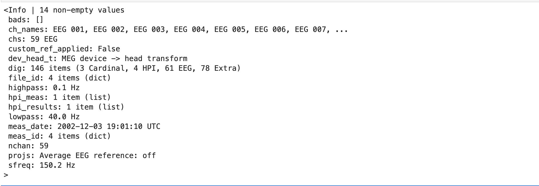
The info attribute keeps track of channel locations, recording date, number of channels, and more. Further detailed information on the Info structure can be found on MNE documentation.
Cropping the Data
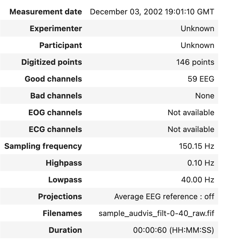
MNE Raw objects have a crop method that can be used to limit the data from the raw file to exist from start-time to end-time (in seconds) which can help save memory. The following code shows how we can crop the data from 0 to 60 seconds:
raw.crop(tmin=0, tmax=60) # crop data from 0 to 60 seconds
Plotting EEG Signals
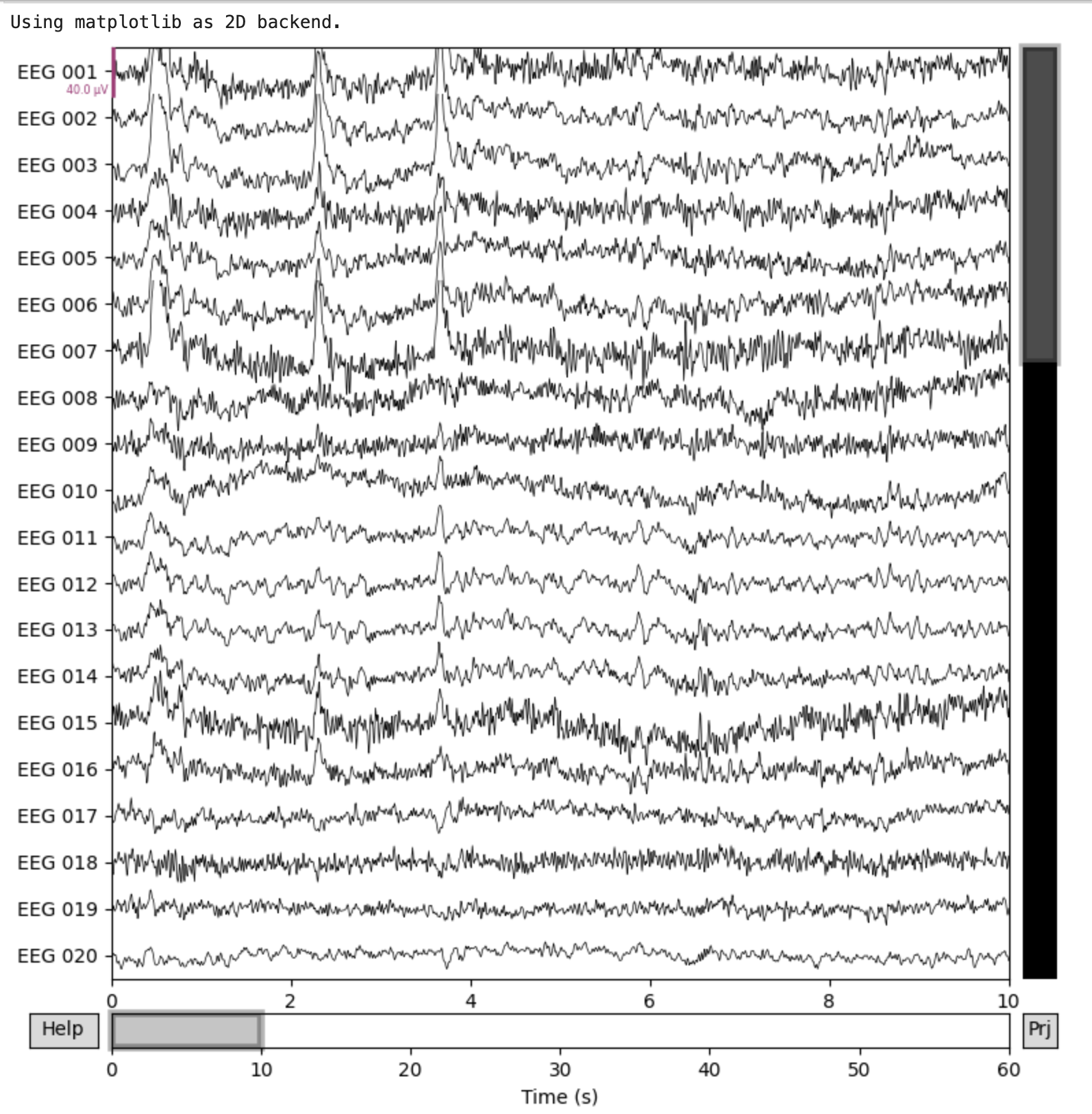
MNE has several methods to plot Raw objects. We can use the .plot() method to generate a plot of the raw data by:
raw.plot()
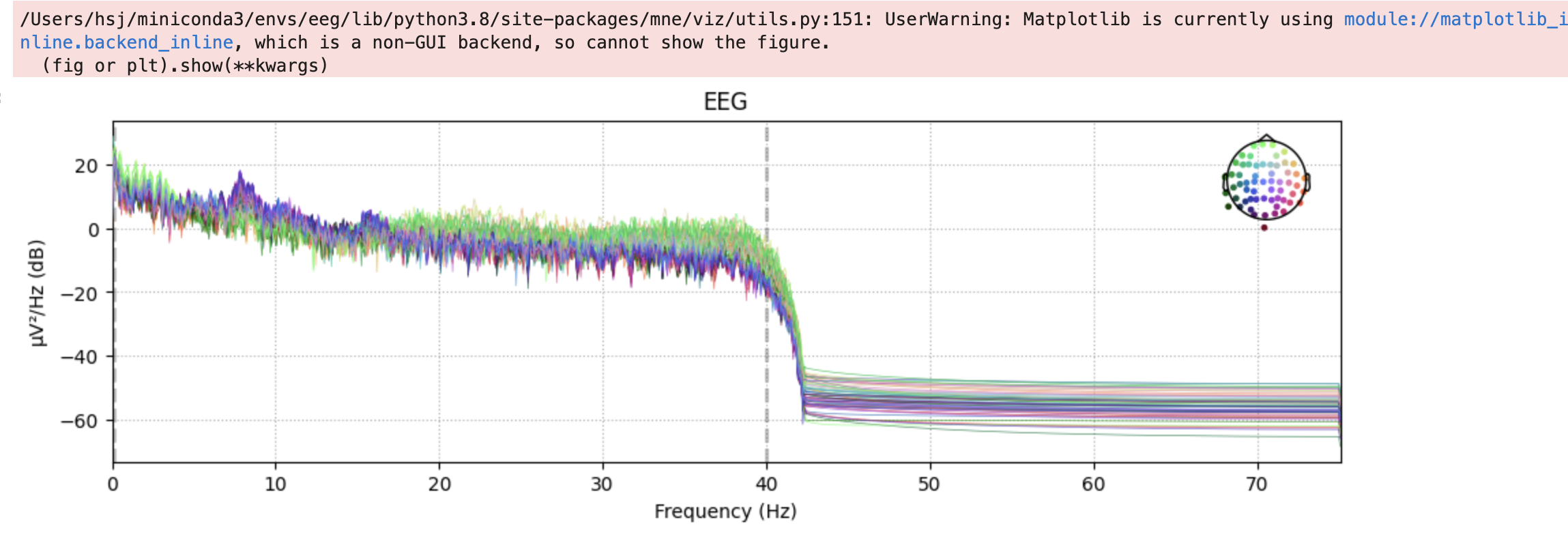
We can also plot the Power Spectral Density (PSD) for each channel. PSD shows the power as a function of frequency and is measured in power per unit frequency. It shows at which frequencies variations are strong as well as at which frequencies variations are weak.
This can be done by:
raw.plot_psd()
Resampling
EEG recordings have a high temporal resolution, so they are often recorded at high sampling rates (eg. 1000 Hz or higher). Although this makes the recordings very precise, it also consumes more memory.
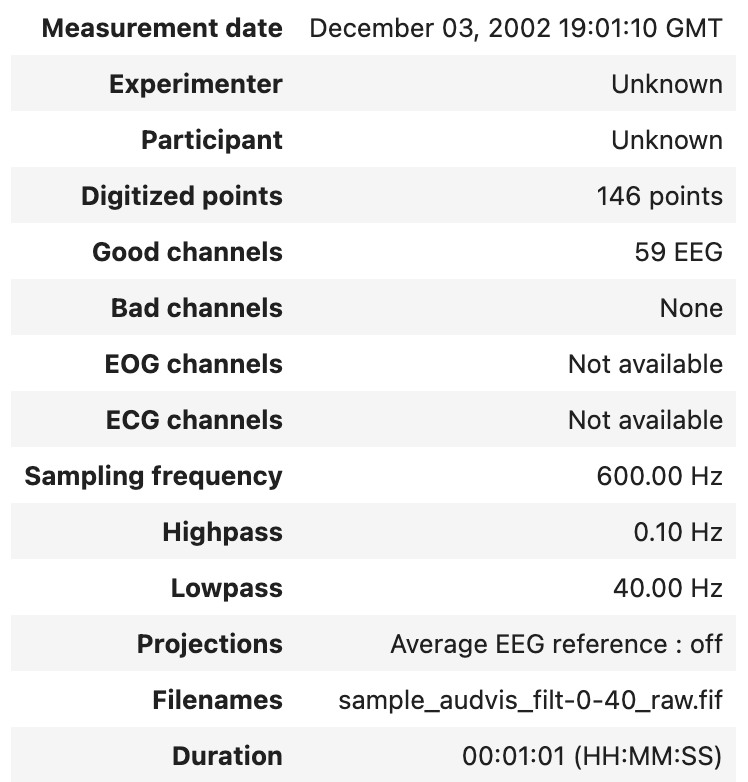
In cases where highly precise timing is not needed, downsampling the EEG signal can help save a lot of computation time. Raw objects have a resample method that can be used to convert from one sample rate to another by:
raw.resample(600) # resample to 600 Hz
Filtering
EEG data can have various artifacts and noise, so preprocessing/filtering must be done in order to maximize the signal-to-noise ratio (SNR), which measures the ratio of the signal power to the noise power. Filtering is one of the techniques used for noise reduction/artifact removal.
Raw objects have a filter method that takes two arguments - lfreq that represents the lower pass-band edge, and hfreq that represents the upper pass-band edge.
High-pass filtering
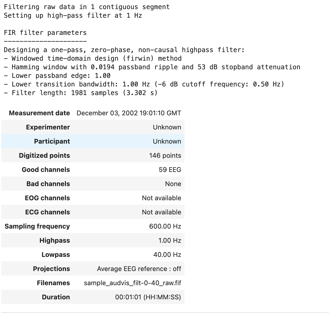
High-pass filtering attenuates frequencies below a certain cutoff frequency. The rest of the signal remains unchanged. The code below filters the signal attenuates the signal below 1 Hz and leaves the rest of the signal unchanged. Since hfreq is None, there is no upper pass-band edge, so the signal is high-passed.
raw.filter(1., None)
Low-pass filtering
Low-pass filtering is essentially the opposite of high-pass filtering. Instead of attenuating parts of the signal below a certain frequency, it attenuates parts of the signal above a certain frequency. It is called low-pass because it lets frequencies lower than a certain cutoff pass.
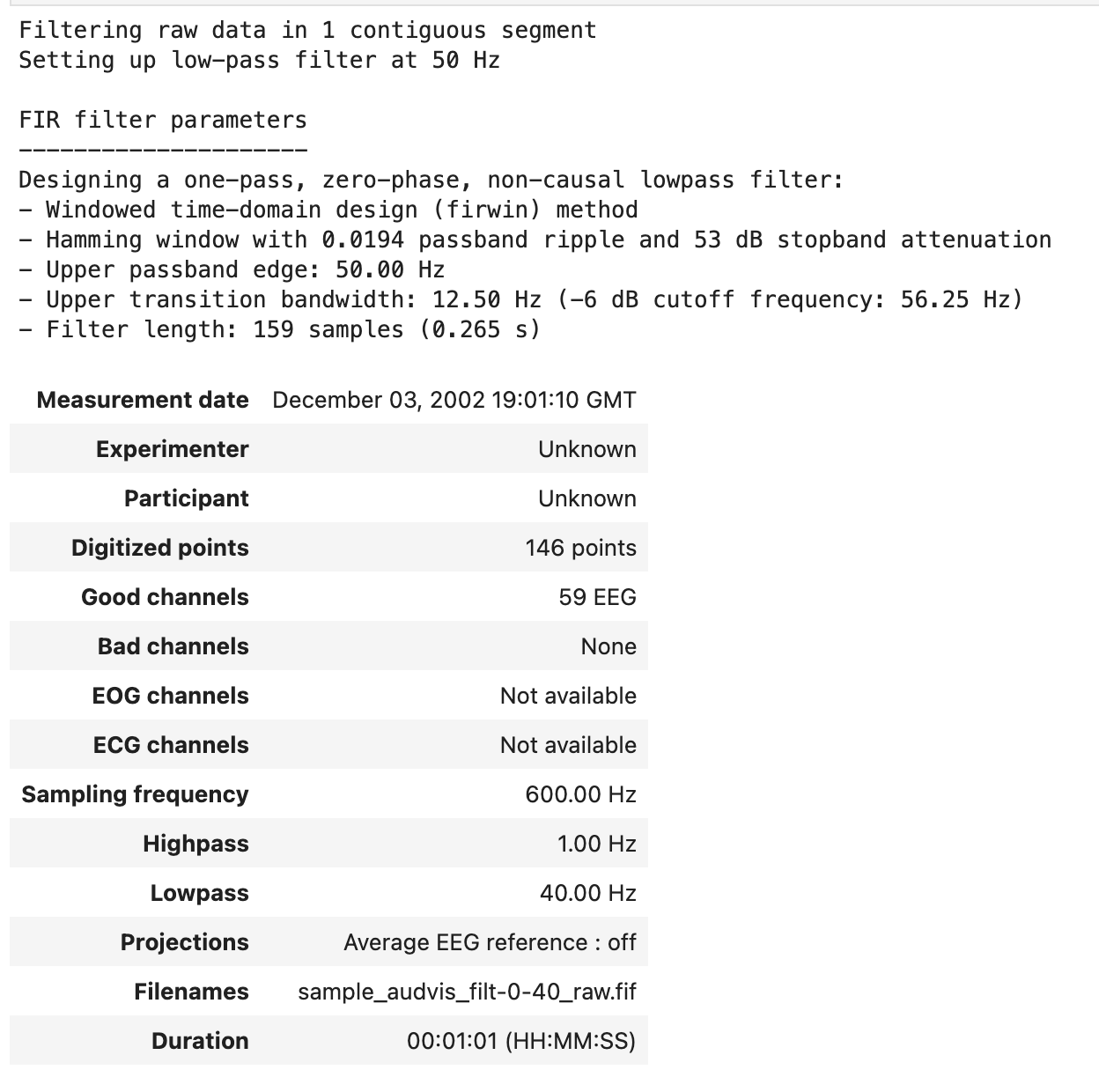
The code below attenuates the parts of the signal above 50 Hz and leaves the rest unchanged. Since lfreq is None, there is no lower pass-band edge, so the signal is low-passed.
raw.filter(None, 50.)
Notch Filter (Band Stop Filter)
The notch filter is a combination of both low-pass and high-pass filters. It can attenuate signals within a specific range of frequencies. The range of frequencies that a band-stop filter attenuates is called the stopband.
Raw objects have a notch_filter method that takes in a specific frequency or a list of frequencies to attenuate the signal at which can be seen in the code below:
raw.notch_filter(50) # attenuate 50 Hz
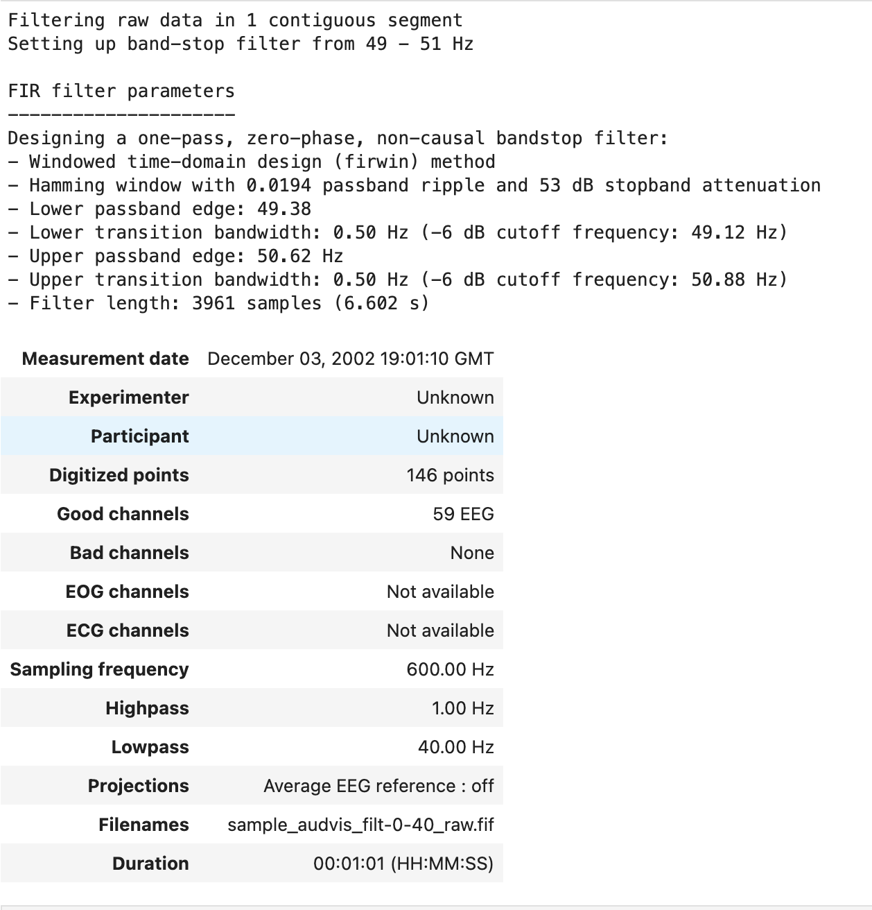
Notch filters are often used when removing power-line noise, which occurs at a frequency of 50 or 60 Hz depending on the recording location. There may be peaks found at the harmonic frequencies, the integer multiples of the the power-line frequency, eg. (60, 120, 180, etc).
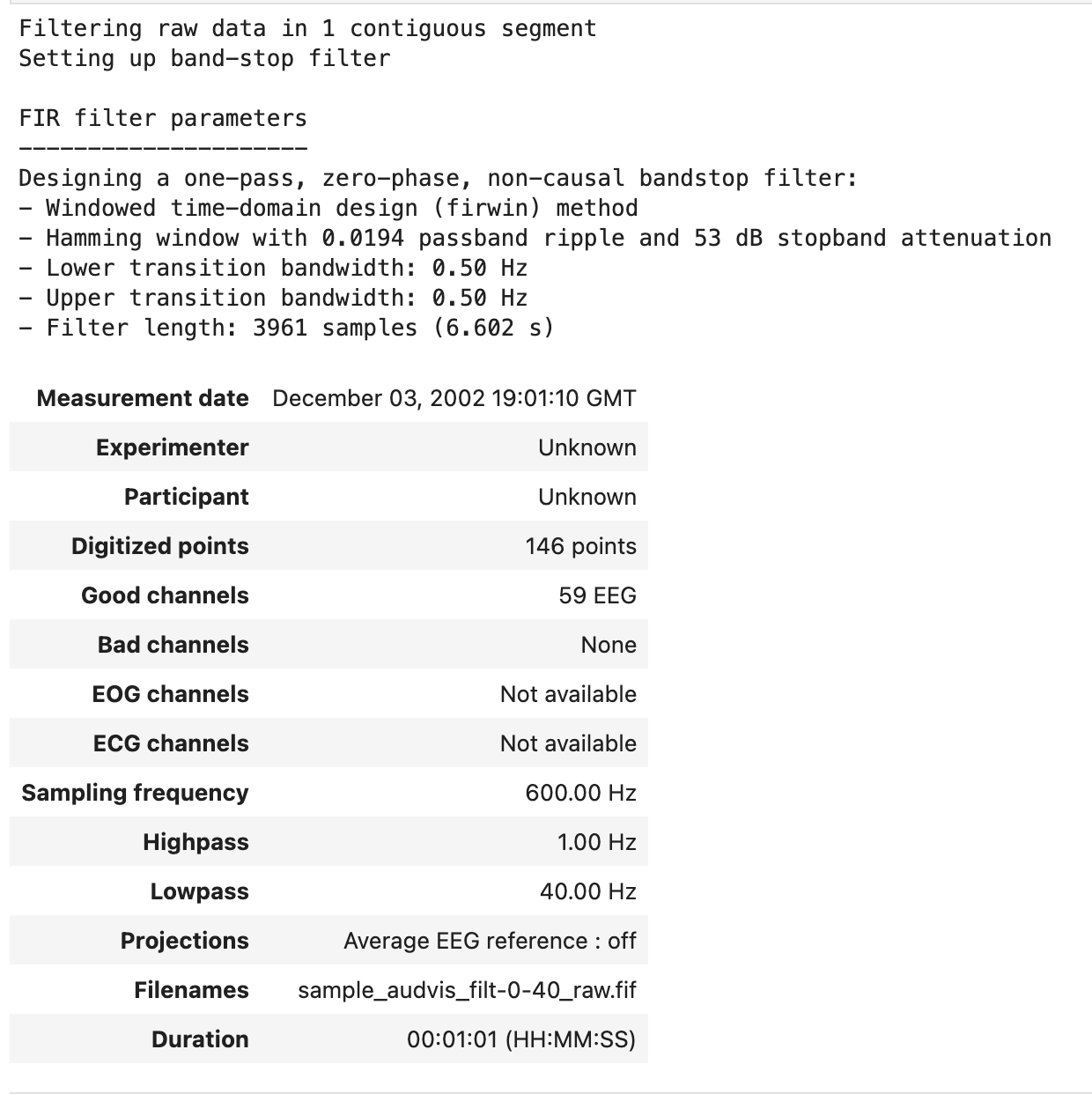
The code below attenuates the signal at 60 Hz and its harmonics.
raw.notch_filter(np.arange(60, 241, 60)) # attenuating 60, 120, 180, and 240 Hz
Epoching
Epochs are equal-length segments of data extracted from continuous EEG data. Usually, epochs are extracted around stimulus events or responses, but sometimes sequential or overlapping epochs are used. MNE has an Epochs object used to represent epoched data. Epochs objects are used in other steps of EEG analysis, including feature extraction, which is used in machine learning.
To create epoched data, MNE-Python requires a Raw object as well as an array of events.
Events
Events in MNE provide a mapping between specific times during an EEG/MEG recording and what happened at those times. Events are stored as a 2-dimensional NumPy array. There are two ways to create events:
- By reading from a file/Raw object or
- By creating equal-sized events.
Reading Events
Lets use a different sample recording because the used before doesn’t contain any events. Therefore:
sample_data_raw_file = os.path.join(sample_data_folder, 'MEG', 'sample', 'sample_audvis_raw.fif')
raw = mne.io.read_raw_fif(sample_data_raw_file, verbose=False)
events = mne.find_events(raw)

Creating equal-length events
Sometimes, there may not be any events included in the raw EEG recording. In such cases, an array of equally-spaced events can be generated. The code below creates second-long events for the first 10 seconds of EEG data:
events = mne.make_fixed_length_events(raw, start=0, stop=10, duration=1.)
Creating Epoched Data from Events
After loading/creating events, creating an Epochs object is fairly simple. preload = True loads all epochs from disk when creating the Epochs object. It can be done by the following code:
epochs = mne.Epochs(raw, events, preload=True).pick_types(eeg=True)

Selecting Epochs
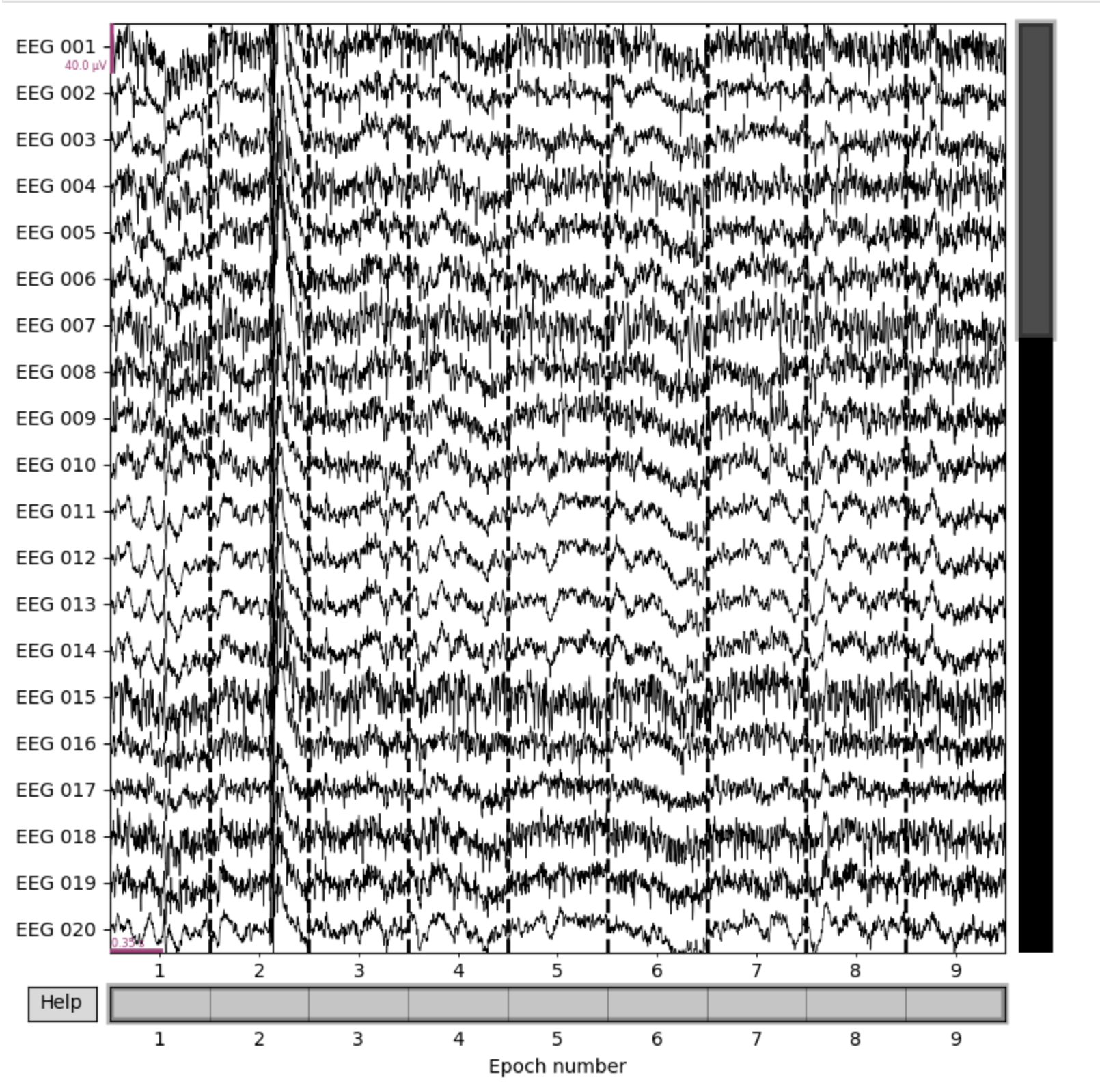
As the Epochs object is now with event labels, one can select epochs using square brackets. For example, one can plot the epochs where the event label was ‘1’ (these event labels have an actual meaning, but they are not shown here for simplicity):
epochs['1'].plot()
Averaging Epochs
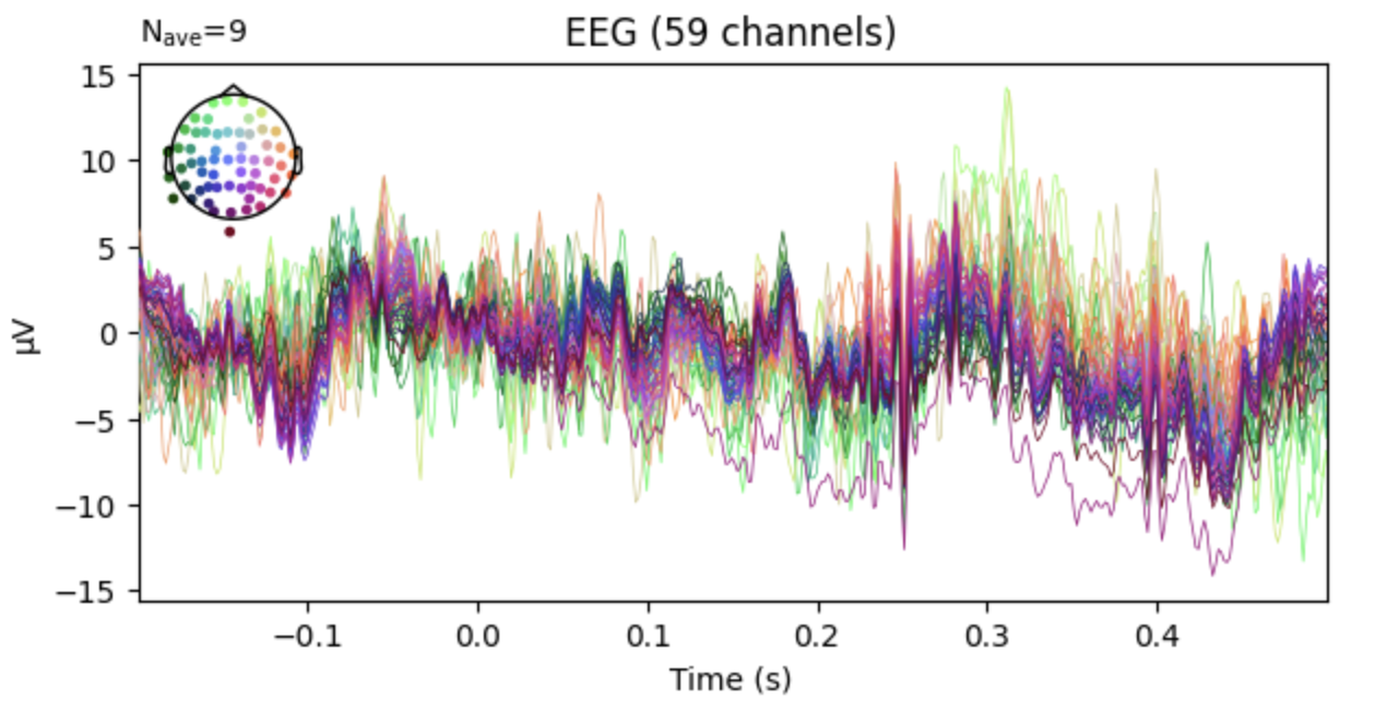
Averaging epochs is a common way to visualize the data. It is done by averaging the epochs across trials. The code below averages the epochs across trials and plots the result:
epochs.average().plot()
Conclusion & Feedback
In this writing, we learned about EEG signals, how they can be loaded, analyzed, preprocessed, and more. Understanding how to process EEG signals is very helpful for tasks such as training a machine learning model to classify EEG segments.
I would love to receive suggestions or any feedback for this writing. It has been written as per my understanding and the learnings I kindled during my journey. I hope you find it useful and easy to understand.