NHL Milestone 1

September 17, 2024

1. Data Acquisition

Objective

In this first section, our objective is to indicate how to get NHL “data” loaded in the memory of a Jupyter notebook. The “data” consists of all the “play-by-play” game events, for ALL NHL games of seasons 2016-2017 to 2023-2024 (including regular and playoffs games!) The “data” is loaded by a Python class; namely the NHLDataProvider class which is explained in the following sections.

1.1 The NHL API and understanding GAME_ID

In brief, to get the play-by-play data of a game, we need to send this GET command, where “GAME_ID” is a unique identifier of a NHL game.

https://api-web.nhle.com/v1/gamecenter/{GAME_ID}/play-by-play

It is important to note that the endpoint above replaces the old API endpoint GET https://statsapi.web.nhl.com/api/v1/game/ID/feed/live after the new API update by NHL.

• Figuring out Game IDs for each season:

  Since we have to download play-by-play events from each game (Regular and Playoffs) from seasons 2016-2017 to 2023-2024, we break-down the logic behind the naming of GAME_ID as mentioned in the following link :
  
  [NHL API Game IDs Documentation](https://gitlab.com/dword4/nhlapi/-/blob/master/stats-api.md#game-ids)
  
  In brief, suppose we take GAME_ID ``` 2019020901 ``` and GAME_ID ``` 2021030217 ``` , the breakdown from left to right would be as follows:
  
  ``` 2019020901 ```
  - '2019' for the season 2019-2020.
  - '02' for regular season.
  - '0901' for game number 901 in the regular season.
  
  ``` 2021030217 ```
  - '2021' for the season 2021-2022.
  - '03' for the playoff season.
  - '0217' -> For playoff games, the 2nd digit of the specific number gives the round of the playoffs, the 3rd digit specifies the matchup, and the 4th digit specifies the game (out of 7). (In this example: 7th game of match #1 in playoff round 2.)
  

1.2 Finding all game Ids of a season

To obtain all the gameIds for each season, our NHLDataProvider class uses the following important private methods:

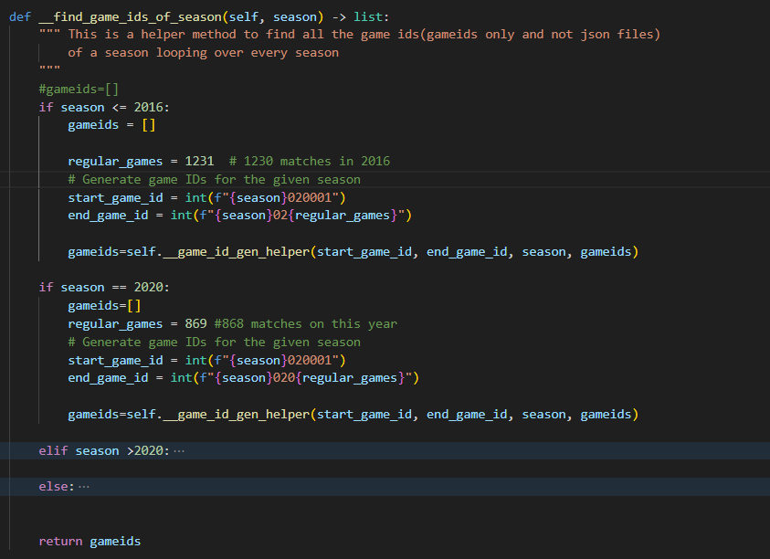
• __find_game_ids_of_season(self, season)
  • This method takes the season as input (ex: season=2018 for 2018-2019) and contains if-else blocks to compute all GameIDs (regular & play-offs) for each season and returns a complete list when called. This is to accommodate for changes in total number of regular games in some seasons, as shown in the figure below.

  

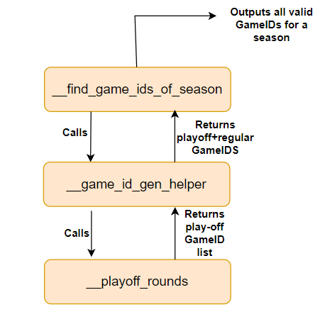
• __game_id_gen_helper(self, start_game_id, end_game_id, season, gameids)
  • This method stores the list of regular games, calls another helper method __playoff_rounds(self,season) to specifically aggregate the valid play-off GameIDs for the season, and returns a list containing all GameIDs for the season back to the __find_game_ids_of_season(self, season) method.
• __playoff_rounds(self,season)
  • This method aggregates a list of valid play-off round GameIDs for the season and returns it back to __game_id_gen_helper(self, start_game_id, end_game_id, season, gameids).

The flow-diagram explains the working of these methods:

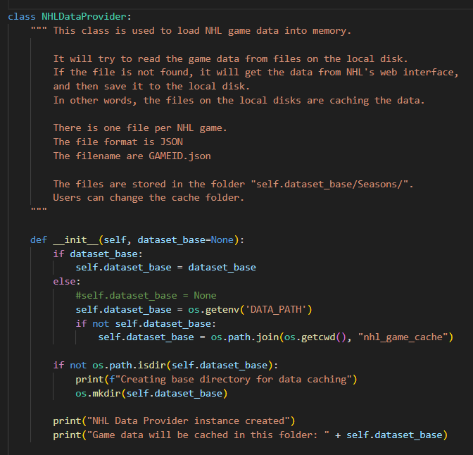
1.3 Understanding the NHLDataProvider Class and how it provides data

The NHLDataProvider class provides public methods to be accessed by the user to return raw data based on the user’s needs. This data is returned either by fetching cached-data or by returning the downloaded data (using the NHL API) when the desired data is not in cache memory.

The initializer of the NHLDataProvider class sets up the cache location as shown in the snippet below:

When the user needs the raw play-by-play data, the class provides two public methods as follows:

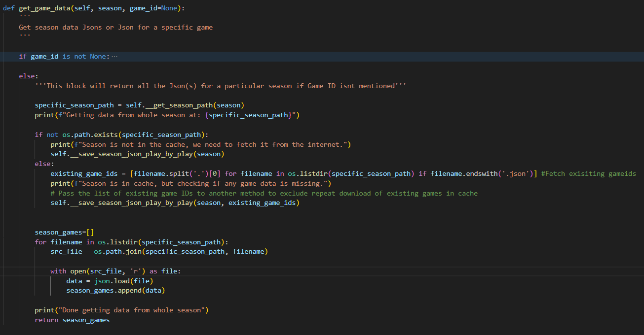
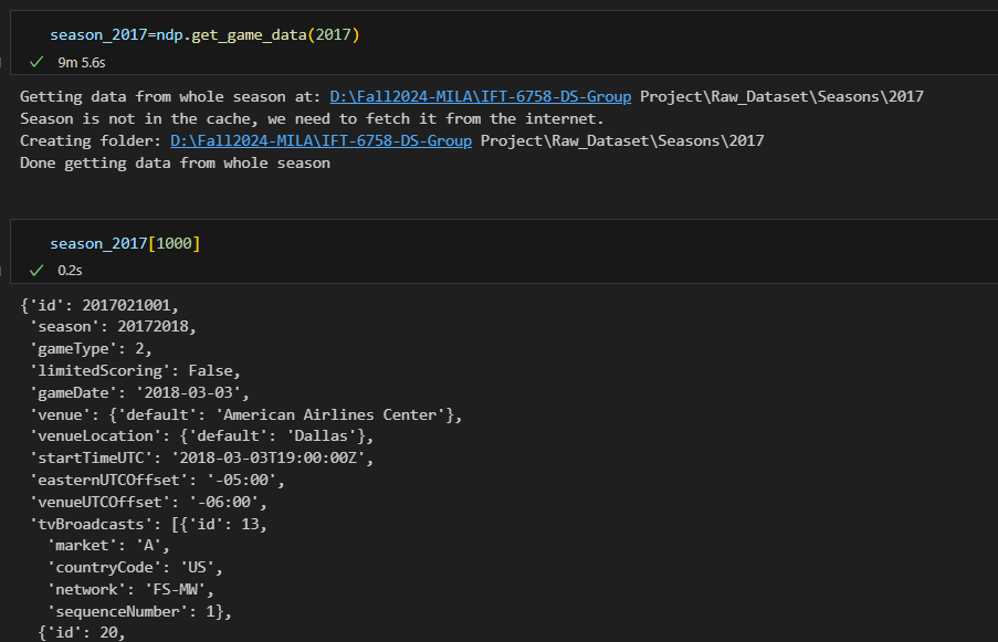
• get_game_data(self, season, game_id=None): This method allows the user to obtain raw play-by-play data in two ways:

  Pass only season: This option allows the user to obtain the raw data by passing only the ‘season’ parameter (example: 2016 for 2016-2017 season). The method also checks if all of the data has been cached already, or if only some games have been cached. If not cached, it will download un-cached data to the desired path (Base_Path\Seasons\2016 for 2016-2017 season for example), and then finally returns the aggregated raw data of all play-by-play events for the season. The snippet below shows the code implementation of this scenario:

  

  Execution in the notebook cell:

  

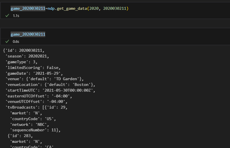
  Pass season along with game_id: This option allows the user to obtain the play-by-play raw data of a specific game, and it also checks if the game_id provided is a valid one. Just like the previous scenario, cached data is returned, else the data is downloaded and then returned.

  

  Execution in the notebook cell:

  

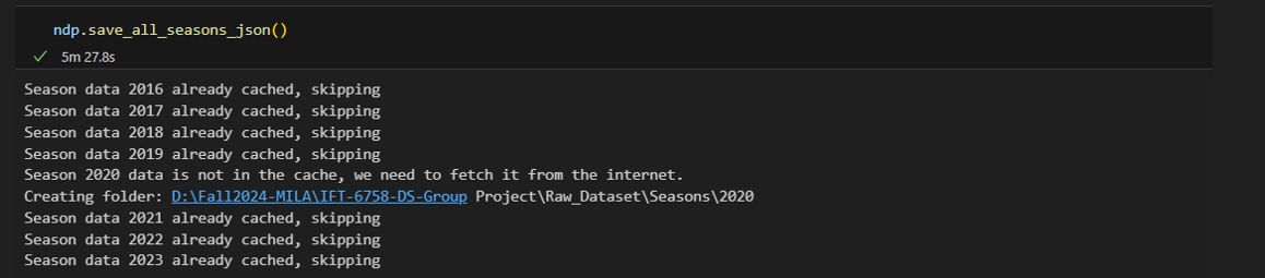
• save_all_seasons_json(self) : This method allows the user to download all the play-by-play data from seasons 2016-2017 to 2023-2024 into appropriate cache paths, while ensuring cached data is not downloaded again. This does not return any data.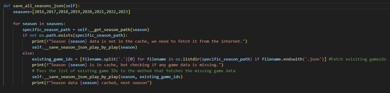

  

  Execution in the notebook cell:

  

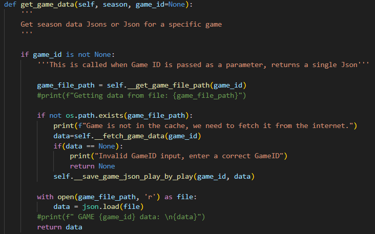
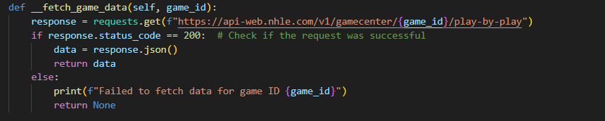
Furthermore, when a game is not cached in memory, the data to be retrieved using the API is called as shown in the following snippet:

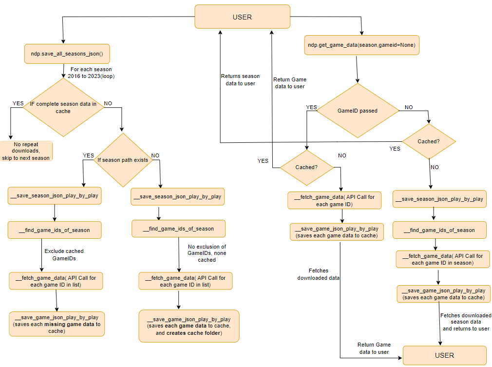
Combining the information from Section 1.2, the following flow-chart explains well the Data Acquisition pipeline:

2. Interactive Debugging Tool

Description of the Debugging Tool

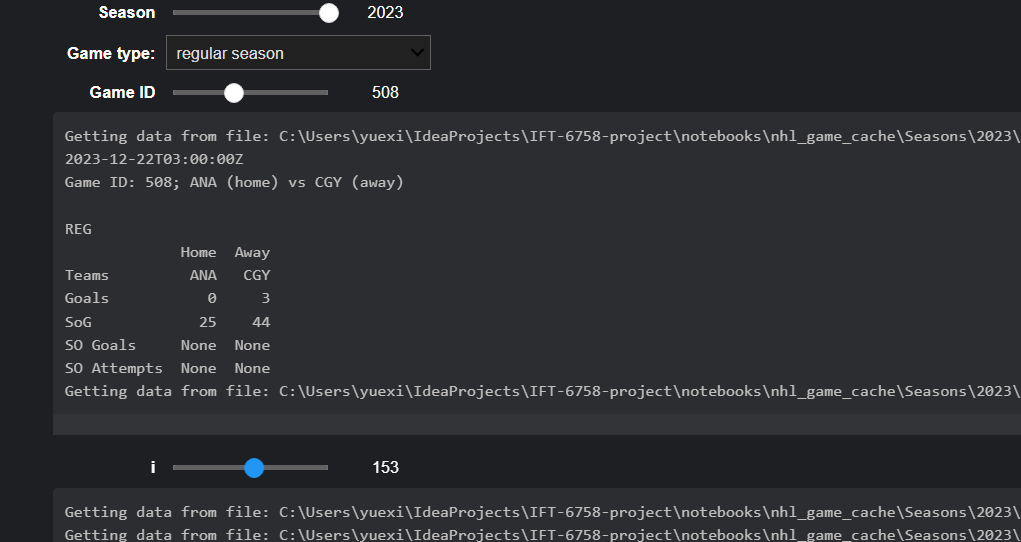
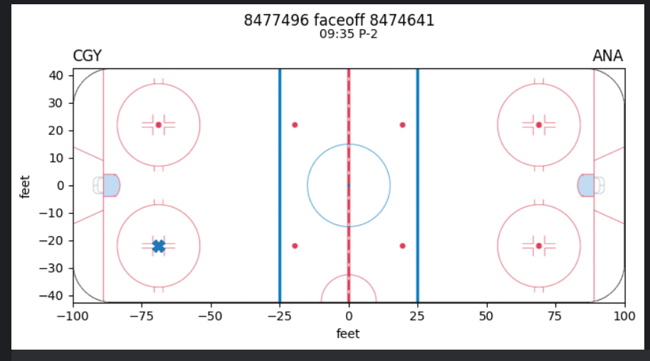
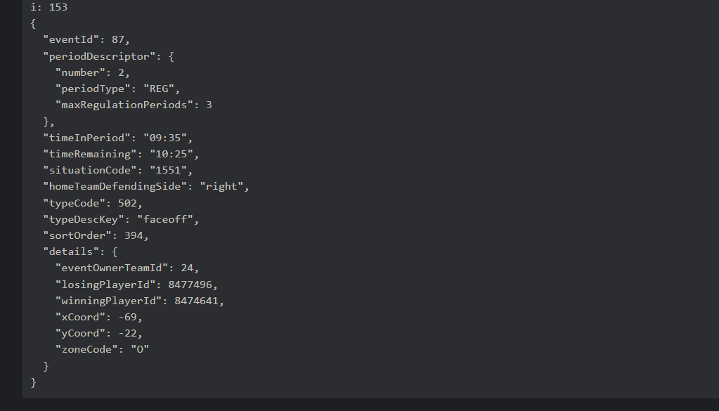
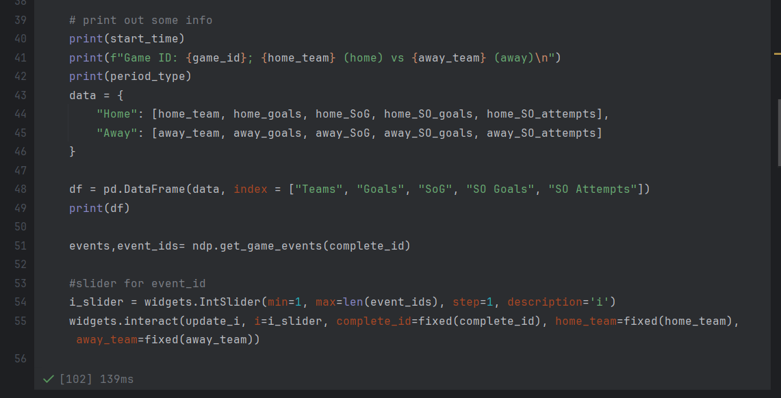
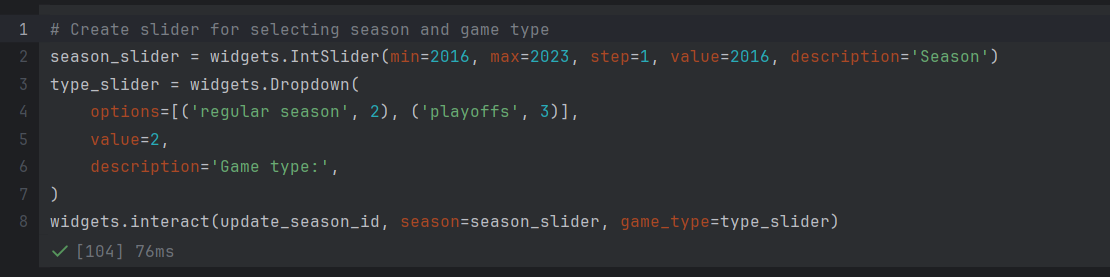
We have implemented 3 widgets for the selection of the game ID: the first slider represents the year, the second, the type of game (regular season or playoffs), and the third, the specific game number. The user is able to select a specific game, and the information about the home team and away team will be displayed. Afterwards, they can choose to view a specific event in the game, where they will see the coordinates of the event on the rink, along with other relevant data obtained from the JSON files.

Screenshots of the Tool

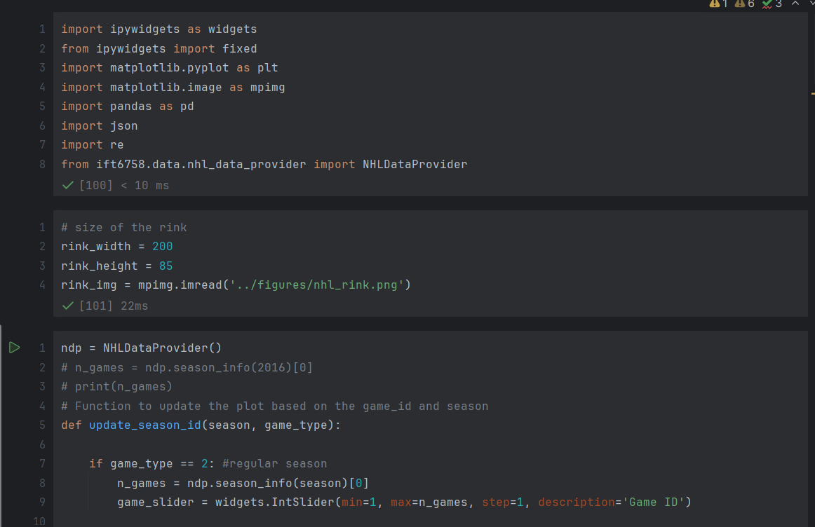
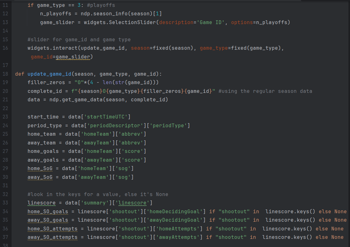
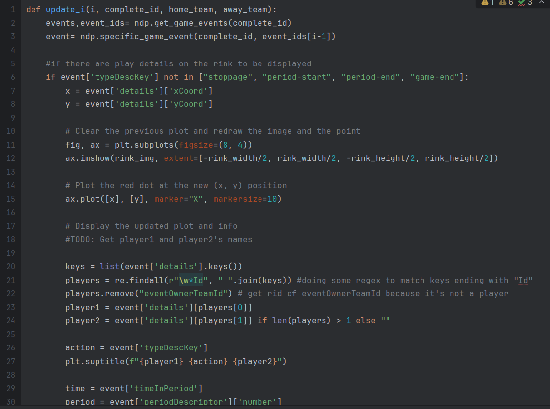
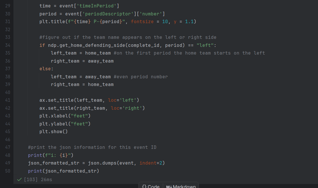
Screenshots of our Code

3. Tidy Data

3.1 Snippets of our final dataframes

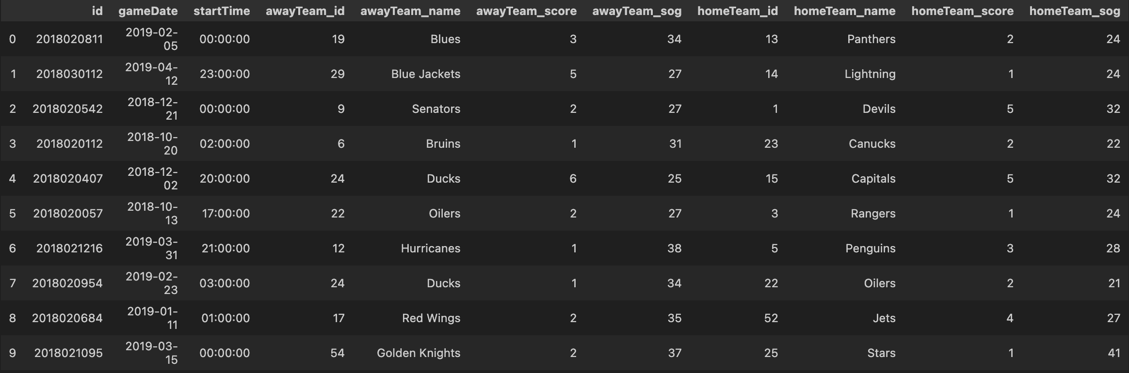
• Season info dataframe
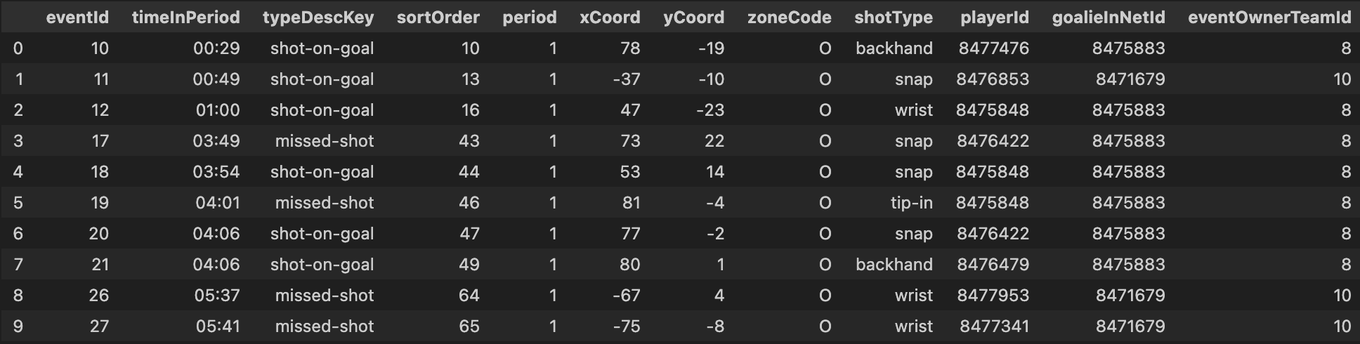
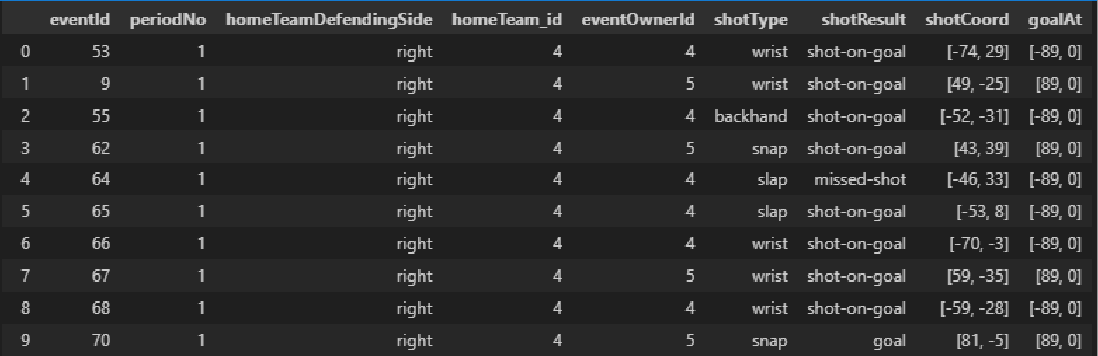
• Shots and goals dataframe This dataframe is used to compute shots information, based on shot types.
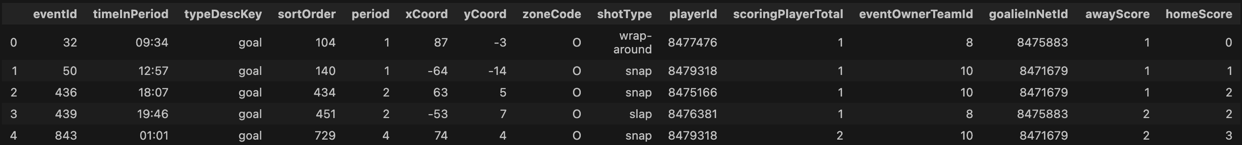
• Goals detail dataframe This is similar to the previous dataframe, filtered to contain only goals
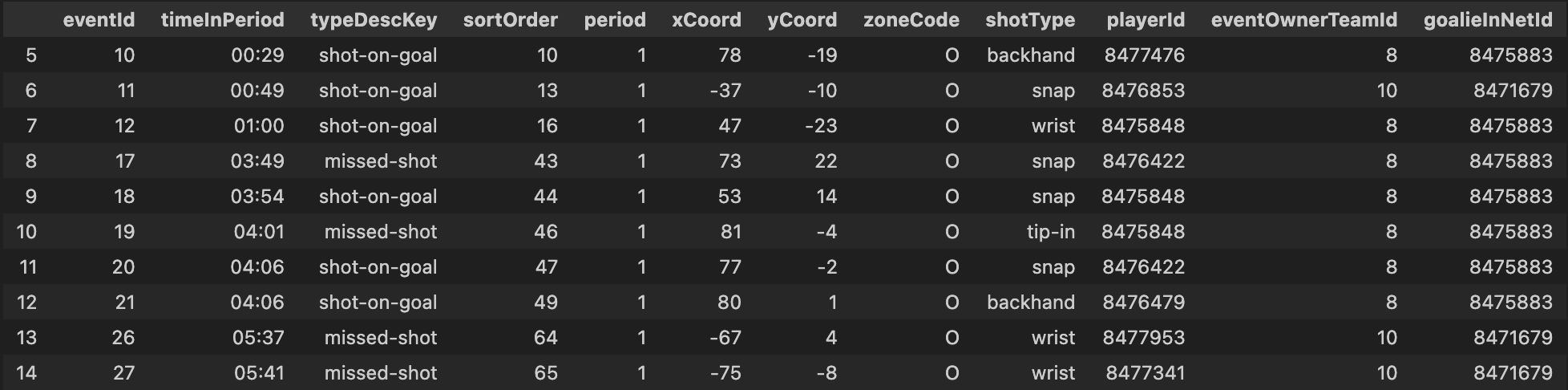
• Shots detail dataframe This is similar to the previous dataframe, filtered to contain only shots without goals
• Shots and Goal Dataframe, with “goalAt” column This dataframe was used to compute the distance between each shots and the target goal. It took longer (about 2-3 minutes) to create this dataframe than the 3 previous ones.

3.3. Suggestion of 3 possible additional features

• According to the previous game, indicate if a scoring/shooting player is in hot/cold streaks; e.g.,
  • if a player has scored more than 2 goals in the last 3 games, we can say that he is in a hot streak
  • if a player has not scored in the last 3 games, we can say that he is in a cold streak
• According to the scoring difference, indicate the game pressure on a goalie
  • if the game scoring is over 2 goals, we can say that the player in behind-team is in a high pressure situation
• According to the blocked shots in opposing team, indicate the defensive pressure on a goalie
  • if the opposing team has blocked more than n shots in the last 5 minutes, we can say that the player is in a high defence pressure situation

4. Simple Visualizations

4.1 Shot types

Important note: for this analysis, we have decided to drop shot types that have been used less than 0.1%, because they don’t represent meaningful information, especially when compared to other shot types. The shot types dropped were “between-legs” and “cradle”, with 0.06% and 0.005% usage, respectively.

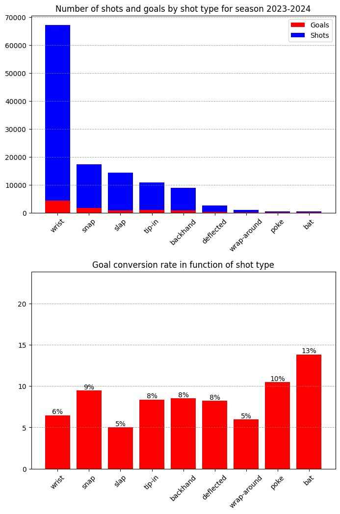Above, we can see 2 bar plots presenting data for shot types of Season 2023-2024. Each bar represent a shot type used by NHL players.

Bar plots are the best visualization method for this kind of data: we can clearly separate the shot-types, while the height of each bar indicates relative information between them.

The top bar plot indicates how many shots and goals were made during the 2023-2024 Season. Note that bar height includes goals (red portion) and the sum of shot-on-goal and missed-shots (blue portion). We can clearly see that the wrist shot is the most used shot type.

The bottom bar plot indicates the percentage of goals for each shot type. From this second bar plot, we can draw interesting conclusions:

• In general, when a player makes a shot, he has around 8% chances to score a goal
• “Snap” shots are a mix of wrist and slap shot. They are more effective (9%) than the wrist and slap shots (6% and 5% respectively). You can have more details about those shot types on the Hockey Monkey web site.
• The most dangerous types of shot seem to be “poke” and “bat” shot type. However, these 2 shot type are not well documented in most hockey analysis web site. We suppose this is because those shot-type are used based on specific opportunities during the game. This means that they happen more often by chance, than by choice of the player. If we concentrate our analysis on shot types selected by players, the snap shot is the most dangerous shot type.

4.2 Goal conversion rate vs distance

Statistics used

As for the previous section, we decided to use 3 types of events to calculate the “Goal Conversion Rate”:

• Goal
• Shot-On-Goal
• Missed-Shot

The “Goal Conversion Rate” is the number of “Goals”, divided by the sum of “Goals”, “Shots-On-Goal” and “Missed-Shots”.

Each of the 3 events contain coordinates of the origin of the shot (XCoord, YCoord). The coordinates are rounded to an integer value (feet). The events also contain a field called “eventOwnerTeamId”, so we can know which team was taking the shot.

NHL Coordinate system

The following image indicates the dimensions of an official NHL ice rink:

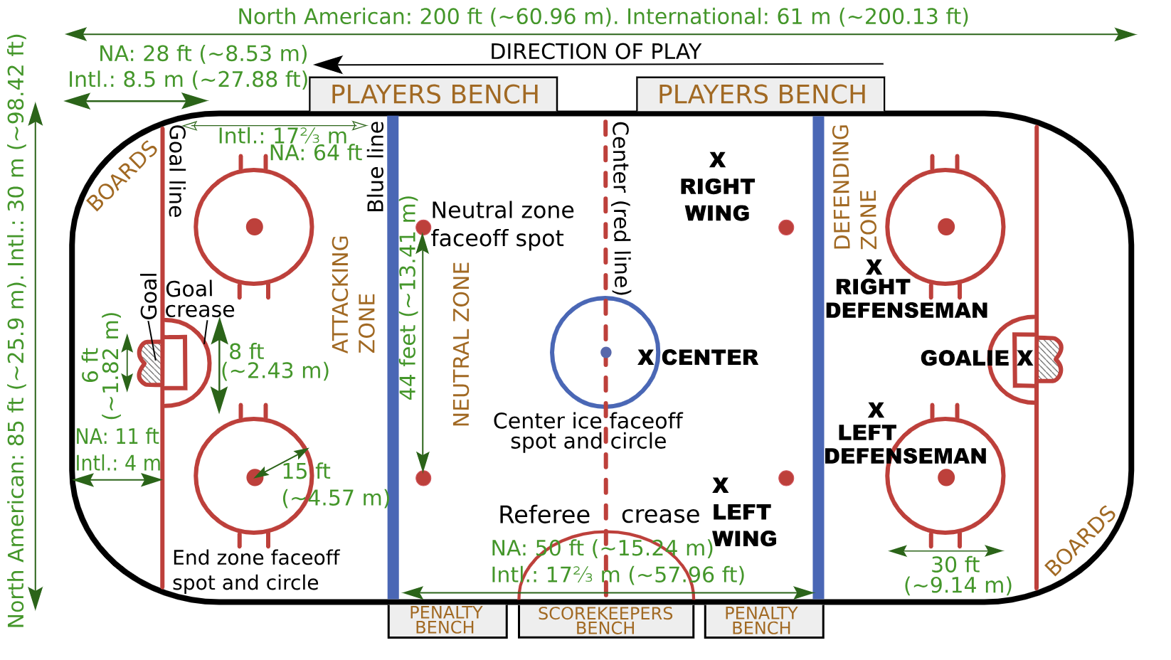
We were able to deduce the following information:

• The origin (0,0) is located at the center of the ice
• The units of the coordinates are in feet
• The rectangular size of the rink is 200’x85’, so the coordinates go from Top-Left (-100, 42.5) to Bottom-Right (+100, -42.5)
• The center of the goals are at: Left goal: (-89, 0) Right goal: (+89, 0)

Challenge of calculating the distance

The distance of a shot is “simply” the Euclidean distance between the origin of the shot and the center of the target goal. However, there is challenge here: we have to find which of the 2 goals is the target goal!

For season 2020 and above, this was quite easy: each game contained a field “homeTeamDefendingSide”. With this information, we could deduce which teamId was on which side at the beginning of the game. For seasons 2019 and earlier, we found that we could look at the first event “shot-on-goal”, for which the zone of “Offensive”. For this shot-on-goal, we look at the XCoord value. If it was positive, it meant that the team taking the shot was aiming at the goal on the right side of rink.

Now that we knew on which side was the “Home Defending Side” at the beginning of the game, we had to be careful to switch the goal side at each period!

Invalid events

When we have parsed the data for seasons 2018, 2019 and 2020, we discovered that some events had bad data. For example, sometimes, the coordinates were missing or had Nan values. Since this represented less than 1% of the events, we decided to just drop those events to complete our analysis.

Results

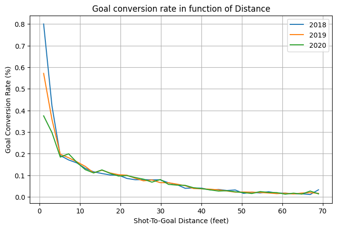
As we can clearly see, the goal rate is inversely proportional to the distance to the goal The results are very similar from one season to another. The reasons are simple:

• The NHL rules have not really changed over these seasons
• We have a lot of data points for each season, so the distribution is very well represented.

The methodology we used to produce this graph is:

• We divided the distance into 35 regions, from 0 to 70 feet (2 feet resolution)
• For each region, we calculated the goal conversion rate
• For each season, we draw a line joining the 35 points of the goal conversion rates.

Filtering shots “too far”

When we started to analyze the results, we found out that shots taken from a distance higher than 70 feet had a “noisy” goal conversion rate. Sometimes, the rate seemed to be higher than shots taken from much closer to the goal. After digging, we understood that

• The goals from distance above 70 (roughly, outside the offensive zone) are rare (< 1 %)
• Those goals were mainly scored in a empty net

So, we decided to remove those goals from our final result graph, because they introduce noise and don’t give meaningful information

4.3 Shot vs distance and shot-type

We have used a similar methodology as in the previous section:

• Remove shots taken from “too far”, which we decided was taken from further than 70 feet.
• Calculate “Goal conversion rate” in bins of 2 feet long
• Remove rarely used shot types (cradle and between-the-legs)
• Force goal conversion rate to 0 when, inside a 2-feet bin, there is only one goal.

Using this methodology really helps to reduce the noise of our figures.

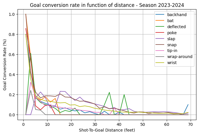
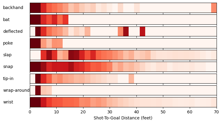
We first started to work only with the top graph, which shows a line for each shot type. We can see some patterns emerging, but it is not very clear where multiple lines cross.

Then, we decided to create a 1D heat-map of the Goal Conversion rate in function of the distance of the shots. The heat-map has colors from white to red, and we saturated the red when the goal conversion rate was higher than 25%. With those heat maps, we better see patterns for the different shot types

• For almost all shot type, when shooting within 5 feet, the chances of scoring a goal are really high.
• The slap shot shows a different pattern than other shot types: it is most effective between 15 and 25 feet. The reason is that a slap shot takes time to be taken: the player must do a long backstroke to take his shot. However, within 15-25, the pucks arrives to the goal so fast that it is really difficult to stop.
• The snap shot seems the most dangerous type of shot. Although its rate regularly decreases when the distance increases, the rate is almost always better than other shot types.

5. Advanced Visualizations: Shot Maps

5.1 Offensive Shot Maps from 2016 to 2020

For the advanced visualisations, we have decided to include missed shots in our calculations to get a more complete picture of offensive performance.

Select the season to display

2016-2017 2017-2018 2018-2019 2019-2020 2020-2021