NHL Milestone 2

November 13, 2024

2. Feature Engineering I

2.1 Histogram of shot counts binned by shot distance and shot angle

NOTE: The ‘Non-Goals’ are shots classified as ‘shot-on-goal’ and ‘missed-shots’ in our data for seasons from 2016-2017 upto 2019-2020(4 seasons). Additionally, shot angles are higher for shots that are taken head-on. For example, a shot angle of 90 degrees means it is directed along the same line as taking a shot from the centre of the pitch towards goal.

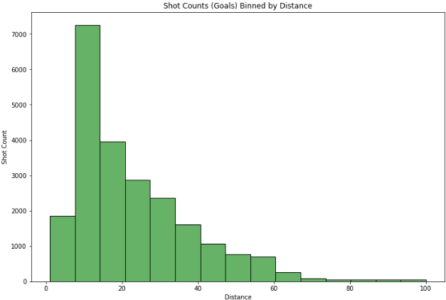
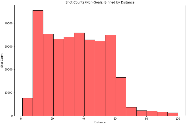
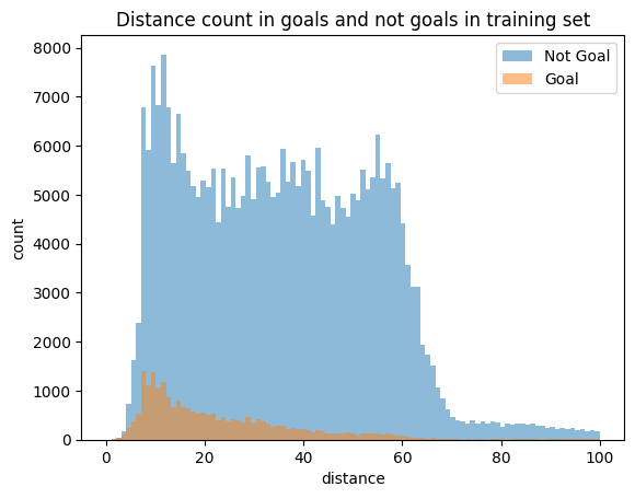
Plotting histogram of shot counts binned by shot distance:

• In the ‘Goals by distance’ distribution, most goal counts cluster around smaller values of distances (0 to 25 feet), with an exponential decrease in counts with increase in distance.

• However, with the ‘Non-Goals by distance’ distribution, the shot counts are more spread out over the range of distances except for very large distances (distance> 60 feet and distance< 10 feet). The shot counts in the 10 to 60 feet range has some resemblances to a uniform distribution.

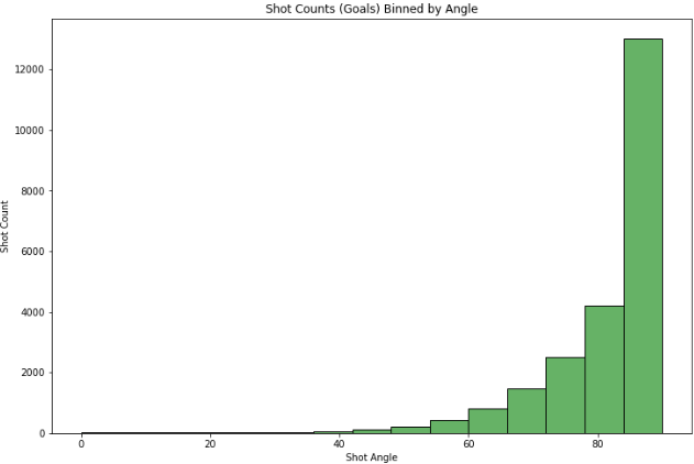
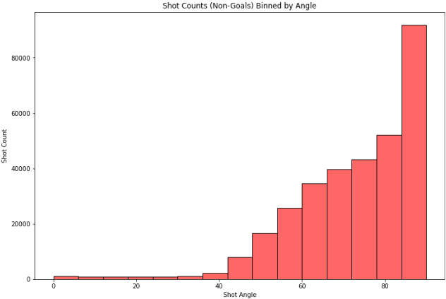
Plotting histogram of shot counts binned by shot angle:

• In the first plot of shots that led to goals versus the angle of the shot, there is an exponential decrease in the in goal count with decrease in shot angle. Most counts are clustered around the 80 to 90 degree shot angle range.

• However in the second plot, there is a smoother decrease in shot counts (like an ascending bell-curve) from the 80 degree mark.

• A common characteristic between the two plots is that there is a large cluster of counts for shot angles >80 and very low counts for shot angles lesser than 40 degrees.

2D histogram of shot distance vs shot angle (goals and non-goals included):

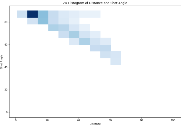
• The darkest (densest) regions are at short distances (0–20 feet) and high shot angles (80–90 degrees).
• This suggests that most shot counts are those taken from close range and directly in front of the net.
• Additionally, the plot indicates also that with increase in distance to the goal, shots are taken at a tighter angles (less head-on towards goal).

References: Joint Plots

2.2 Plotting Goal Rate (Goal/(No Goals + Goals)) binned by distance and shot angle

Goal rate by shot distance:

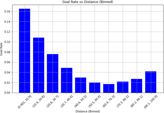
Observations

• The highest goal rates occur in the smallest distance bin ( 0–10 feet), with a goal rates exceeding 0.16. Generally the goal rates are higher for smaller distances from goal.

• There is an exponential decline in goal rate as the distance increases (0 - 60 feet). Beyond 40 feet, the goal rate becomes very low (below 0.05), indicating that long-range shots have much lower chances of success.

• From the 80 feet range (80 - 100 feet), there seems to be a slight increase in goal rate over distance. This is potentially due to the presence of wrong data(wrong x, y coordinates) in contrast to the actual events of the game, which is explained further in section 2.3.

Goal rate by shot angle:

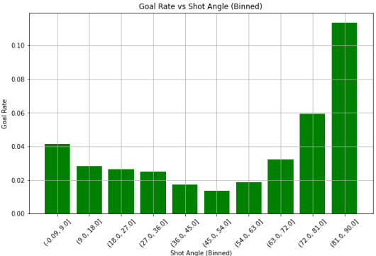
Observations

• The highest goal rate is observed in the largest shot angle bin (80–90 degrees), with a goal rate above 0.10. These are most likely head-on shots directly in front of the goal.

• Another slight rise in goal rate is seen at small angles (0–10 degrees), possibly reflecting odd deflections or rebounds.

• The goal rate is significantly lower at intermediate shot angles (e.g., 20–70 degrees), with values clustering around 0.02–0.05. These shots are among the least likely to be goals possibly due to ease at which saves can be made.

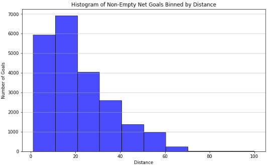
2.3 Plotting Histograms of empty and non-empty goals

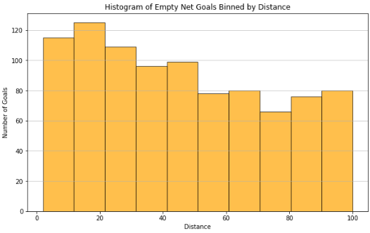
Observations

• It is easy to observe that the counts of goals scored as ‘Empty net’ goals are much lower (max count is 120 in a bin) than the counts of goals in ‘Non-empty’(max count of 7000 in a bin) goal situations, across the 4 seasons. This implies that Empty net situations are not a common occurrence.

• There is a resemblance in the shape of the distribution between the two plots for distances between 0 and 20 feet. However after this mark, the numbers of goals scored on ‘Non-Empty’ goals sees a steep decline in count, which makes sense as it is harder to score a long range goal towards a guarded net.

• This is in contrast to the distribution of goal counts beyond 20 feet for ‘Empty Net’ situations-although there is a decrease in goal counts with increase in distance, it is much more gradual, indicating that scoring a goal at an ‘Empty Net’ does not get too much harder with an increase in distance.

Investigating long distance goals on ‘Non-Empty’ goals

• The plot for ‘Non-empty’ goals shows a very small count for goals scored beyond 80 feet, however - still not 0. Upon further investigation, a few gameIds were investigated and we found that some goal entries had mislabelled X and Y coordinates for goals both in the raw JSON data extracted using the NHL play-by-play API and even on the play-by-play plot for the event on the NHL GameCenter website for the same game.

We present two examples as proof of this scenario:

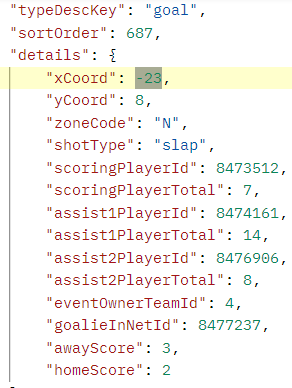
• GAME ID 2016020349

The JSON entry and the Official NHL play-by-play plot for the long distance (shot taken near defensive zone) ‘Non-Empty’ goal is shown below:

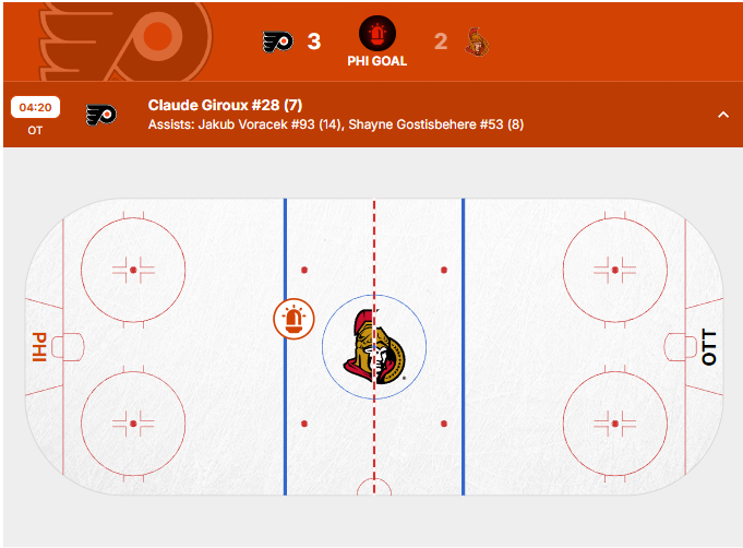
However, the actual goal was scored from a different coordinate:

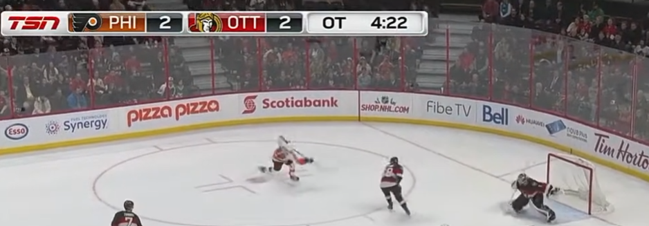
The replay of the game and the actual event can be seen at the 6:05 mark in this video

• GAME ID 2017020870

Official NHL play-by-play plot for the mislabelled goal:

Actual goal was scored from near range:

The actual moment of the game can be seen at the 3:05 mark in this video

3. Baseline Models

3.1 Accuracy

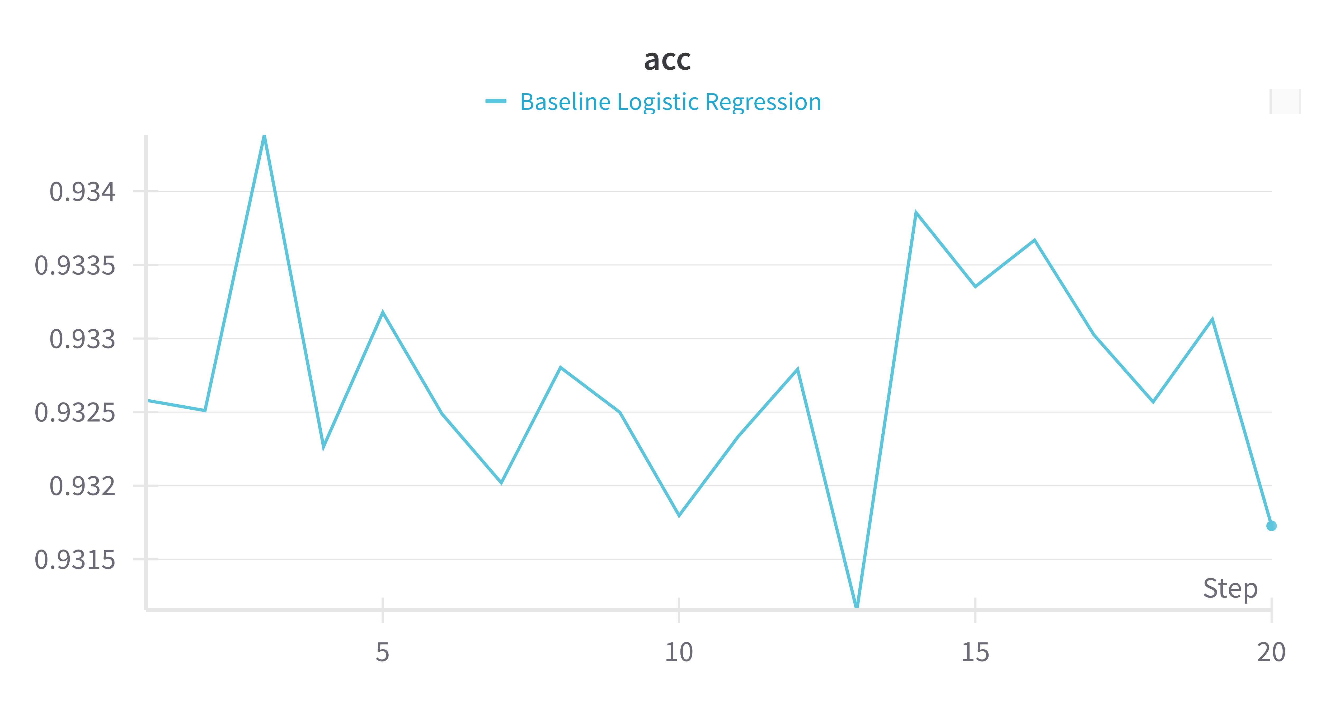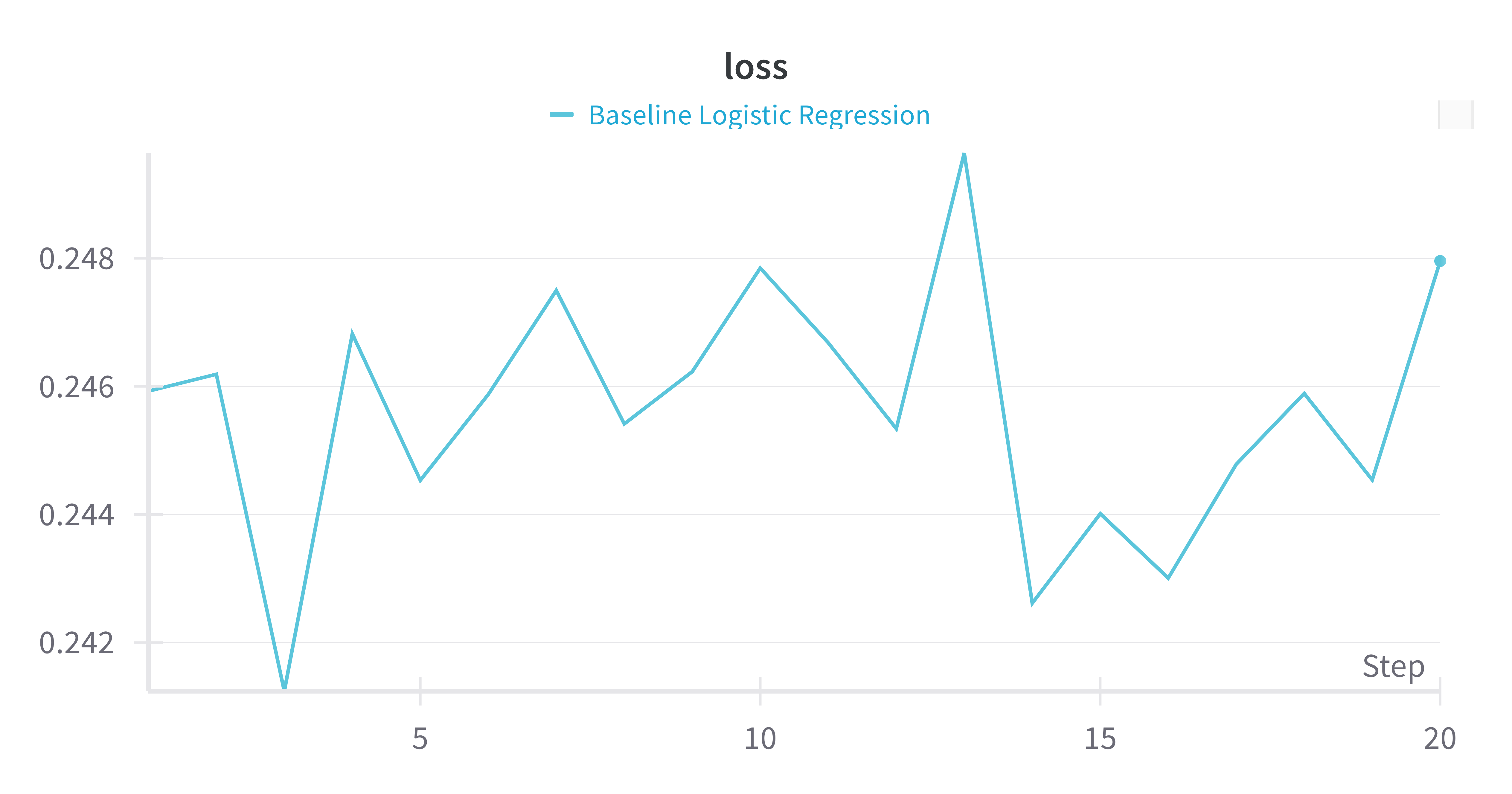In this simple logistic regression model, we do 20 times of cross validations. From the above 2 plots in loss and accuracy, we can see that the accuracy and loss look “seemingly good”. The accuracy is around 0.93 and the loss is around 0.24. However, the prediction proportion of goal and non goal is abnormal.

Steps	Count of Goal prediction	Count of Non goal prediction
Step 1	0	85510
Step 2	0	85510
Step 3	0	85510
…	…	…
Step 20	0	85510

All the predictions are non goals while the accuracy is still high. The model cannot generalize the outcome of goal and non goal as the model doesn’t produce any prediction on the goal.

The potential issue is that the performance metric does not provide a valid evaluation of the model, masking high variance due to:

• Feature limitation: the model is too simple to capture the complexity of the data. Using only the distance cannot capture all necessary information to predict if a goal will be scored.
• Class imbalance: the number of goals and shots are biased, which makes the model biased towards the majority class (not a goal).
• Threshold limitation: the model is not able to predict the goal as the threshold is not set specifically. The threshold is set to 0.5 by default, which is not suitable for this scenario.
• Model limitation: the logistic regression model is not suitable for this task as it is a linear model and the relationship between the features and the target is possibly non-linear.

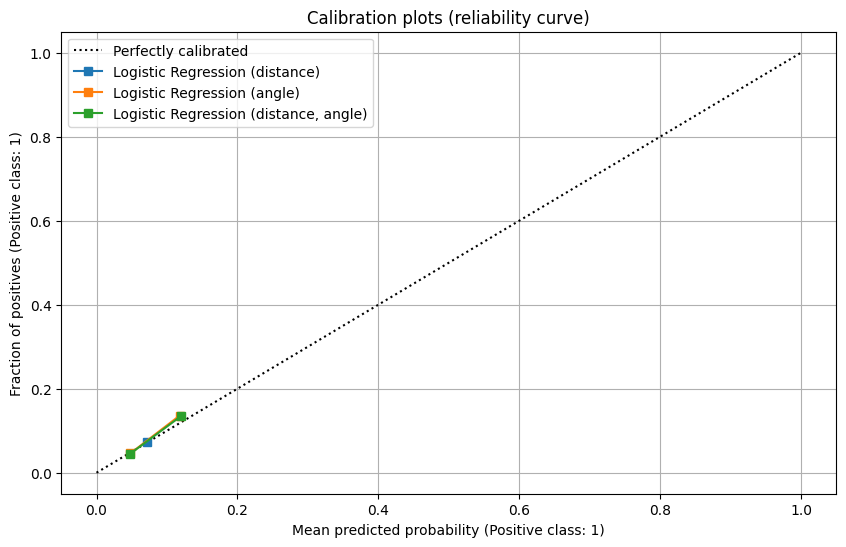
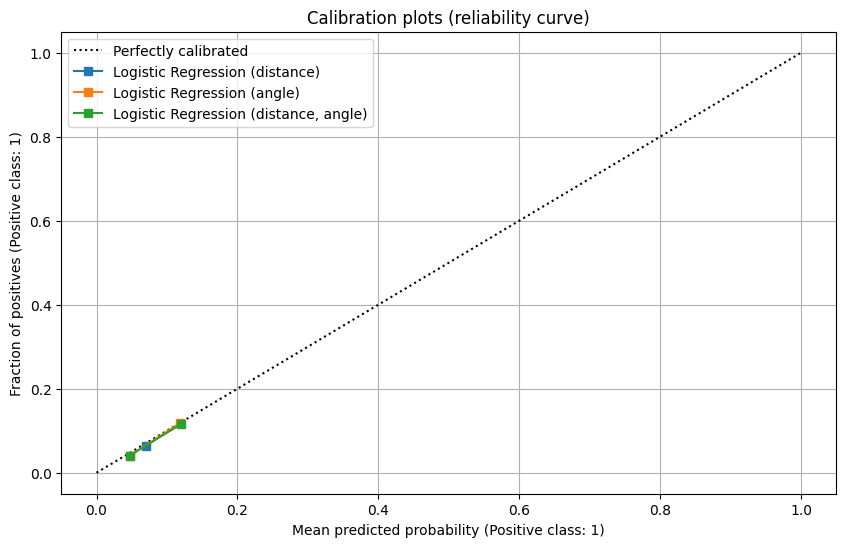
3.3 Base Model plots

Links:

• Experiment 0_Logistic Regression (distance)
• Experiment 1_Logistic Regression (shotAngle)
• Experiment 2_Logistic Regression (distance, shotAngle)

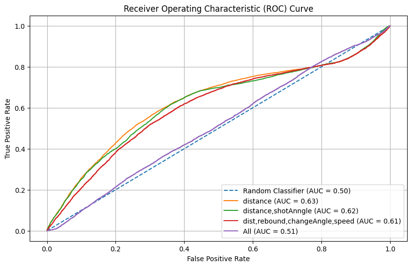
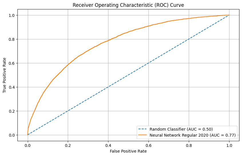
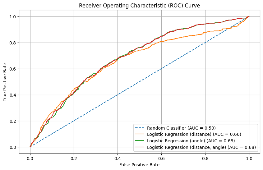
From these 4 plots, we can see

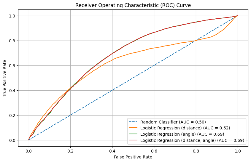
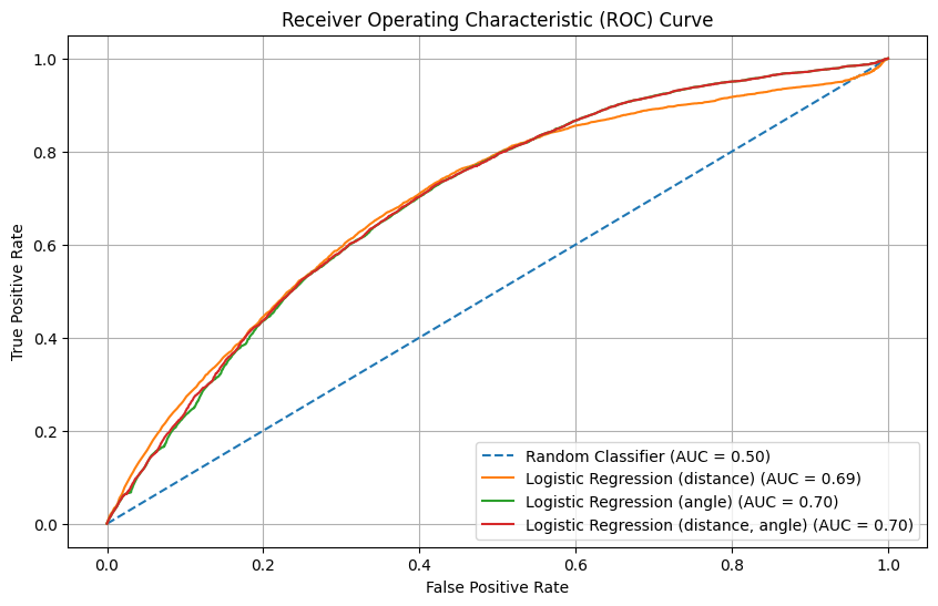
• The ROC AUC curve
  • The model using only distance has the worst performance (AUC = 0.62), while the models with angle only and with both distance and angle perform similarly (AUC = 0.69).
  • At a false positive rate (FPR) above 0.8, the model using only distance performs even worse than the random classifier, suggesting poor reliability in high FPR scenarios.
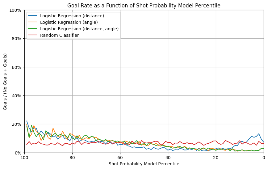
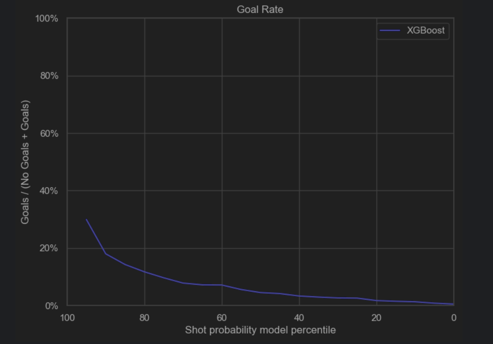
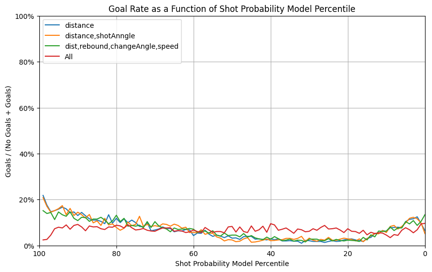
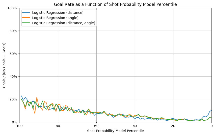
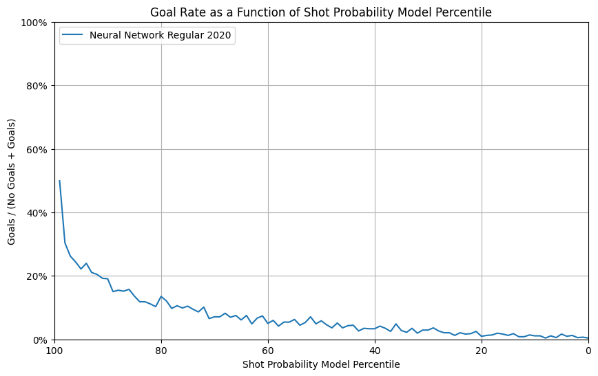
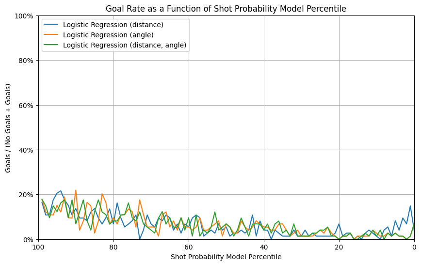
• The goal rate vs probability percentile plot
  • The random classifier exhibits a flat and low goal rate across percentiles, reflecting its lack of predictive power.
  • The model using angle only has a peculiar increase in goal rate for shot probabilities below the 20th percentile, which could indicate overfitting or irregular calibration in this range.
  • All the baseline models, generally show a general trend of increasing goal rate as the predicted probability percentile increases.
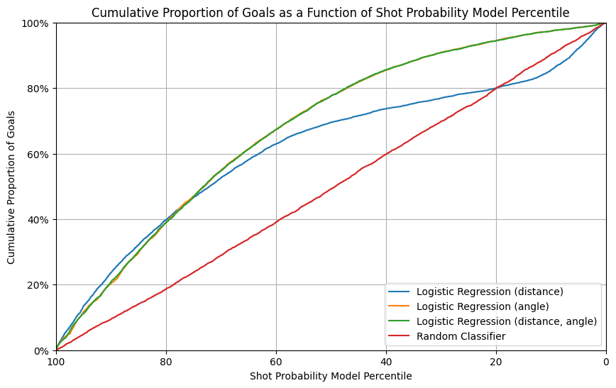
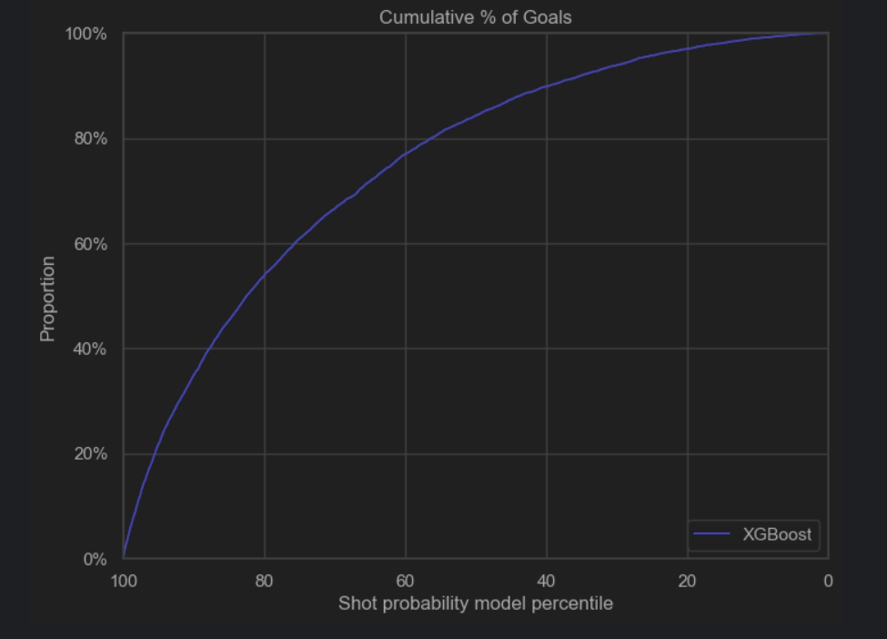
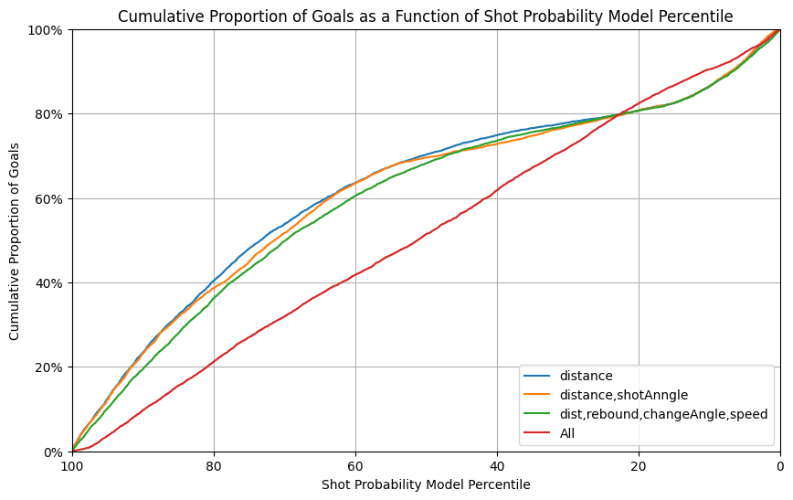
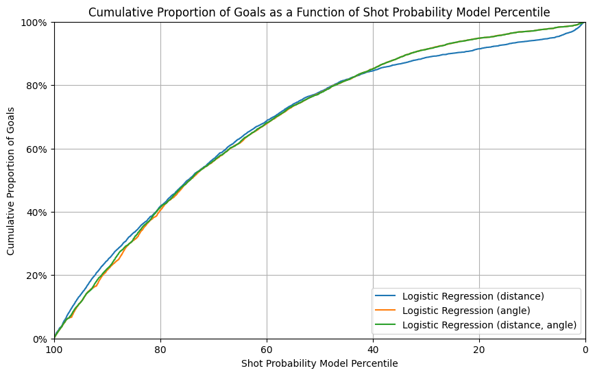
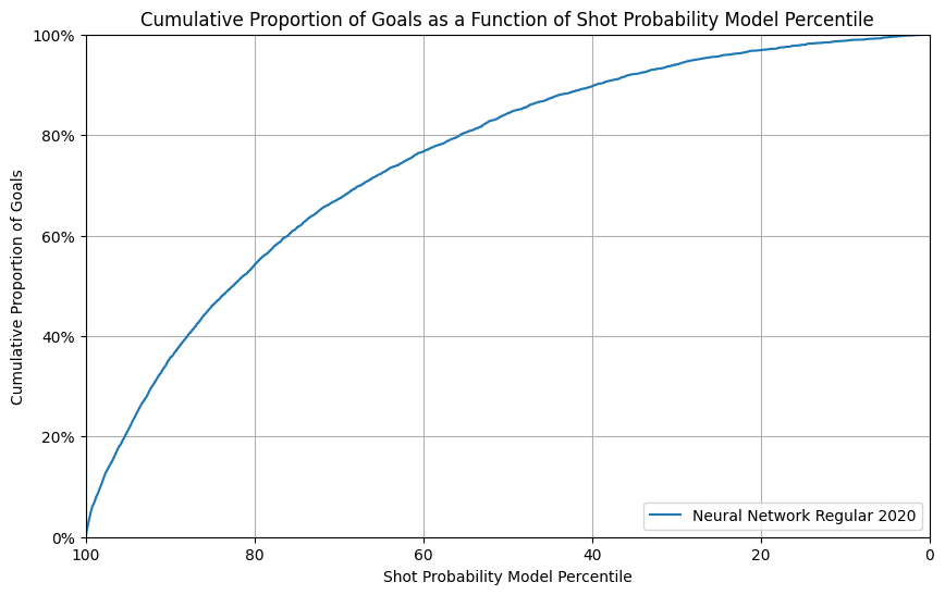
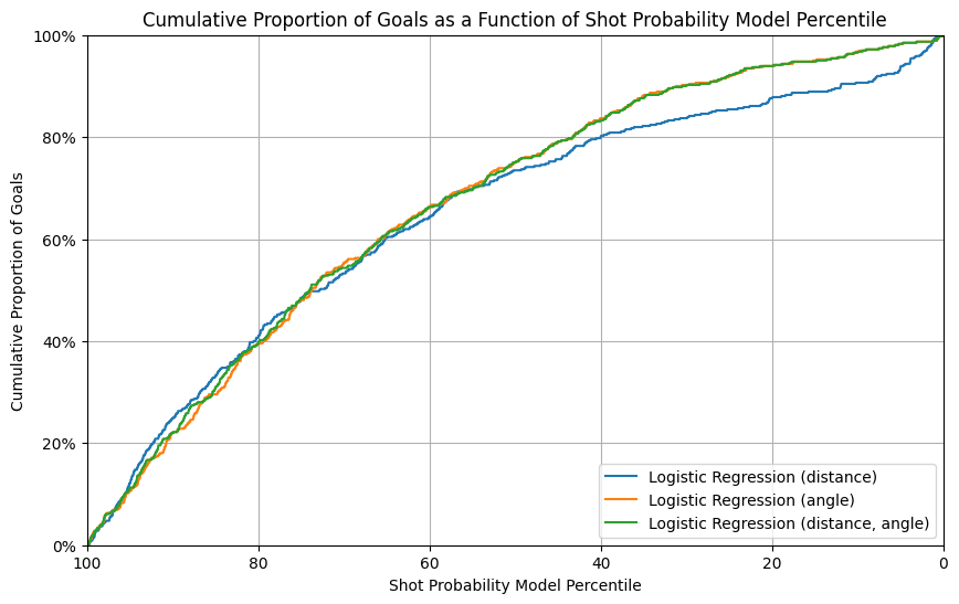
• The cumulative proportion of goals vs probability percentile plot
  • The cumulative goal plot aligns with the trends seen in the ROC curve, showing that models using angle (alone or combined with distance) outperform the model with distance only.
  • The random classifier trails significantly behind the other models, as expected.
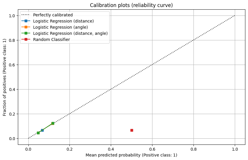
• The reliability curve
  • All baseline models show limited calibration with predicted probabilities confined to a narrow range, though they align on the “perfectly calibrated” diagonal.
  • The random classifier’s calibration is notably poor, with predictions far from the perfect calibration line, further affirming its unsuitability for this task.

The model using only distance performs the worst, while the models using angle (alone or combined with distance) demonstrate comparable and better performance. This indicates that angle is a more significant feature than distance in predicting goals.

The random classifier is ineffective as it lacks any meaningful predictive tendencies or calibration.

The rise in goal rate at low percentiles for the distance-only model indicates potential issues with calibration or feature representation that require further investigation.

4. Feature Engineering II

Basically, we created the features suggested in sections 4.1, 4.2 and 4.3 of the assignment.

Dataset logging into W&B

Team B4 Dataset experiment in W&B

Feature	Description
Distance	Distance between the current shot and the target goal
shotAngle	Angle of the current shot to the goal (90 deg is straight line, 0 deg is beside the goal)
shotType	Type of current shot taken
isEmpty	1: indicates that there was no goaler in the target goal when the current shot was taken
lastEventType	Type of the event that occurred before the current shot
timeSinceLastEvent	Time (in seconds) since the last event
distFromLastEvent	Distance (in feet) between the current and the previous events
rebound	1: Indicates the current shot is a rebound from the previous shot
changeInShotAngle	Difference of angle between the current shot and the previous shot
speed	Estimated speed of the puck between current and previous shots (assuming straight line)

5. Advanced Models

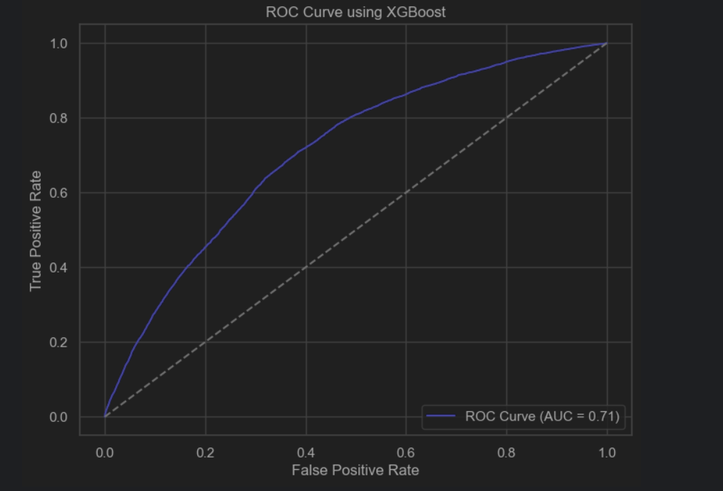
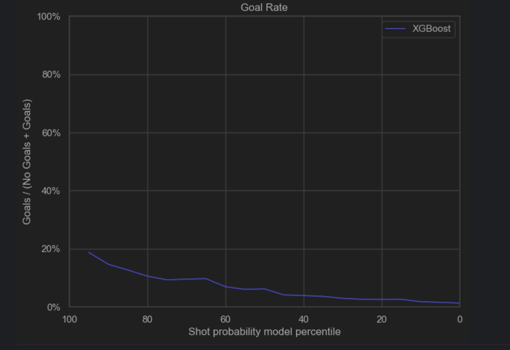
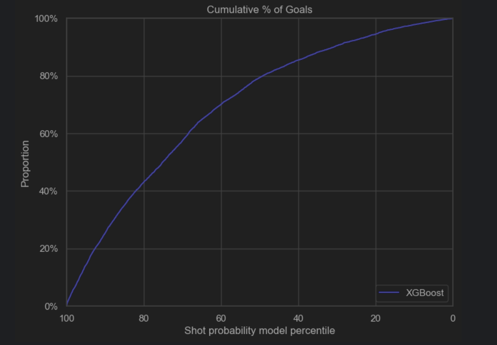
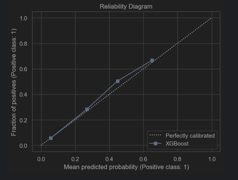
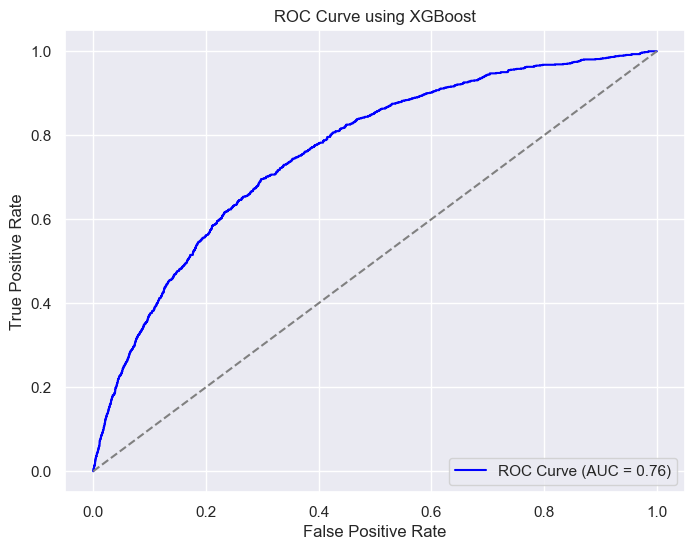
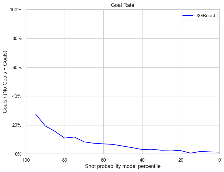
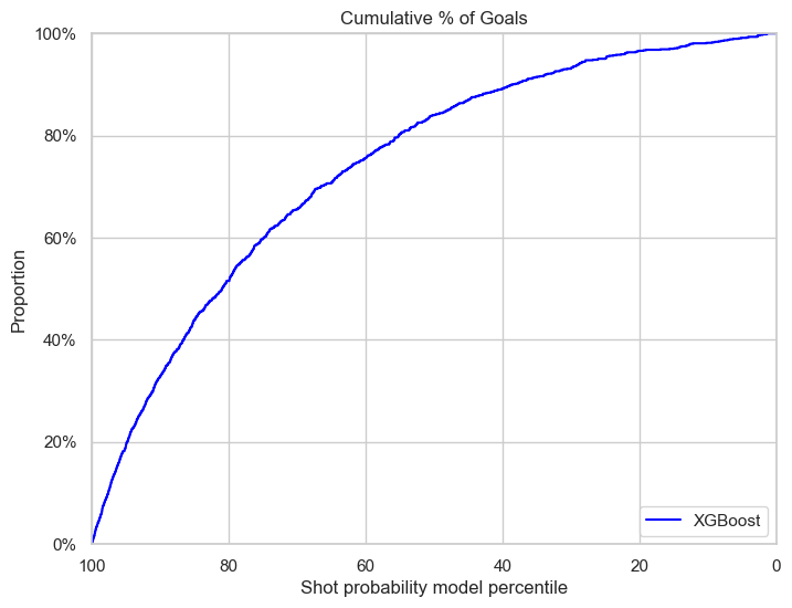
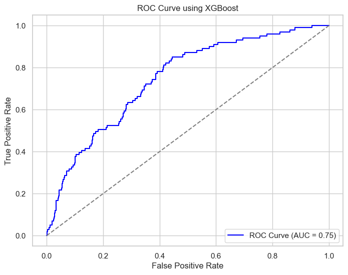
5.1 Simple XGBoost Model

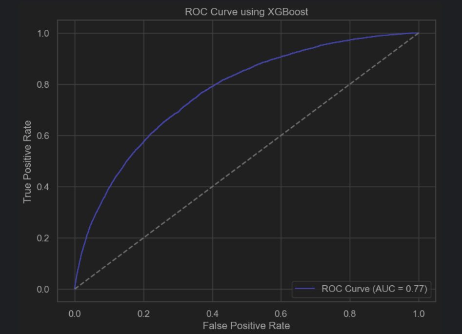
The simple XGBoost model was implemented using the xgboost library in Python and no parameter passed to the model. For our dataset, we used the data from the regular seasons from 2016-2016 up to the 2019-2020. The dataset was divided between train and test, with the test set being 20% of the total dataset. For the training set, the rows containing NaNs were dropped, as the same data would be used for feature selection and certain functions did not support NaNs. The test set was left untouched, since it would be more similar to the real test set. String features such as ‘shotType’ and ‘lastEventType’ were encoded to integers using a label encoder from scikit. The simple model scored 0.934 on accuracy and 0.710 for auc, which is slightly better than the best logistic regression model that had an accuracy of 0.93 and an auc of 0.69.

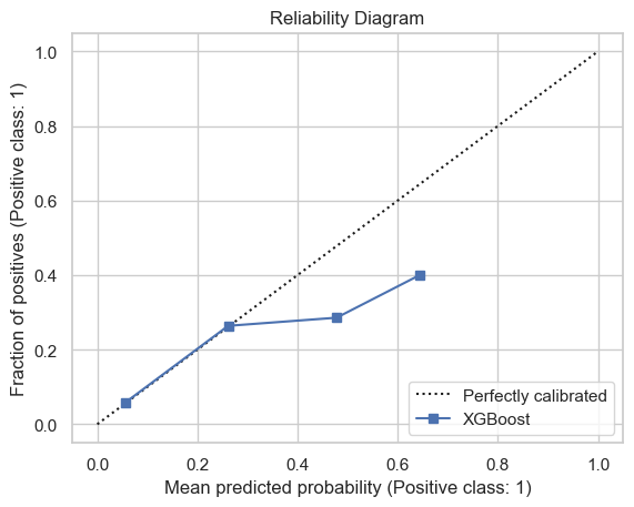
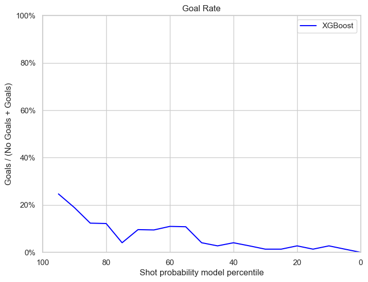
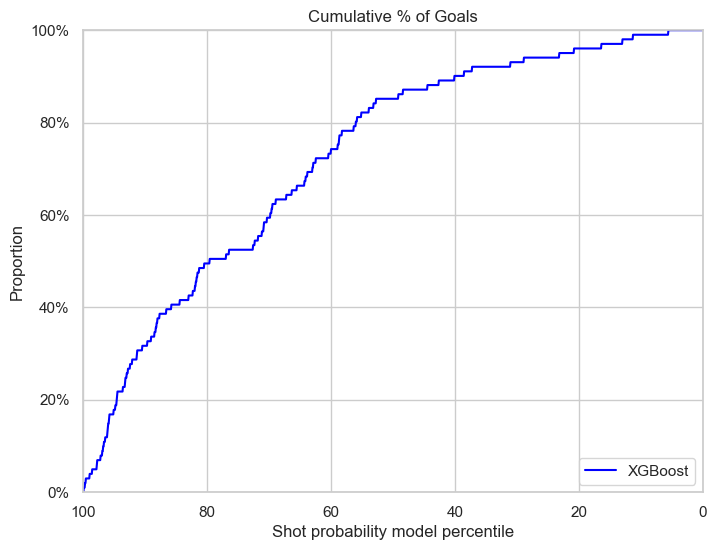
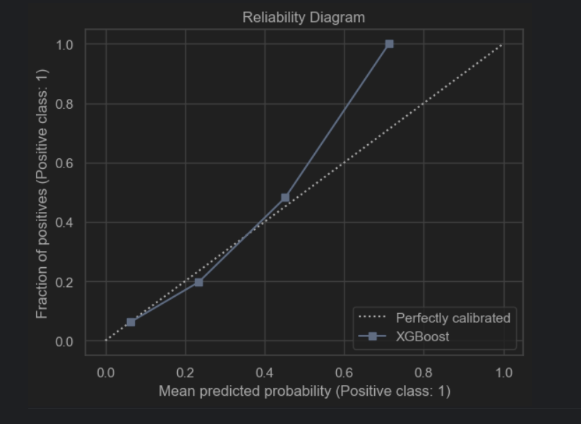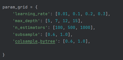
5.2 Hyperparameter Tuning

Experiment Setup

To perform hyperparameter tuning on XGBoost, GridSearch with cross-validation was used. We have also included all the features extracted from part 4. Since limited resources were available, we tried to optimize the choice of hyperparameters and the setup. More hyperparameters were given to the parameters that might more influence on the performance, such as ‘learning_rate’, ‘max_depth’ and ‘n_estimators’. The search also included other parameters such as ‘subsample’ and ‘colsample_bytree’, but only two hyperparameter were given. Cross-validation was limited to two layers to avoid excessive numbers of compute. The metric chosen for the tuning was roc_auc due to the dataset being unbalanced. In the end, the tuning involved 192 candidates, totalling 576 fits. Here is are our choices for the values of the hyperparameters:

Results of Hyperparameter Tuning

After performing hyperparameter tuning, the performance of the model increased: the roc_auc score went up to 0.765 and the accuracy remained 0.931. We plotted some heatmaps to see the impact of pairs of the most important hyperparameters on the auc_score.

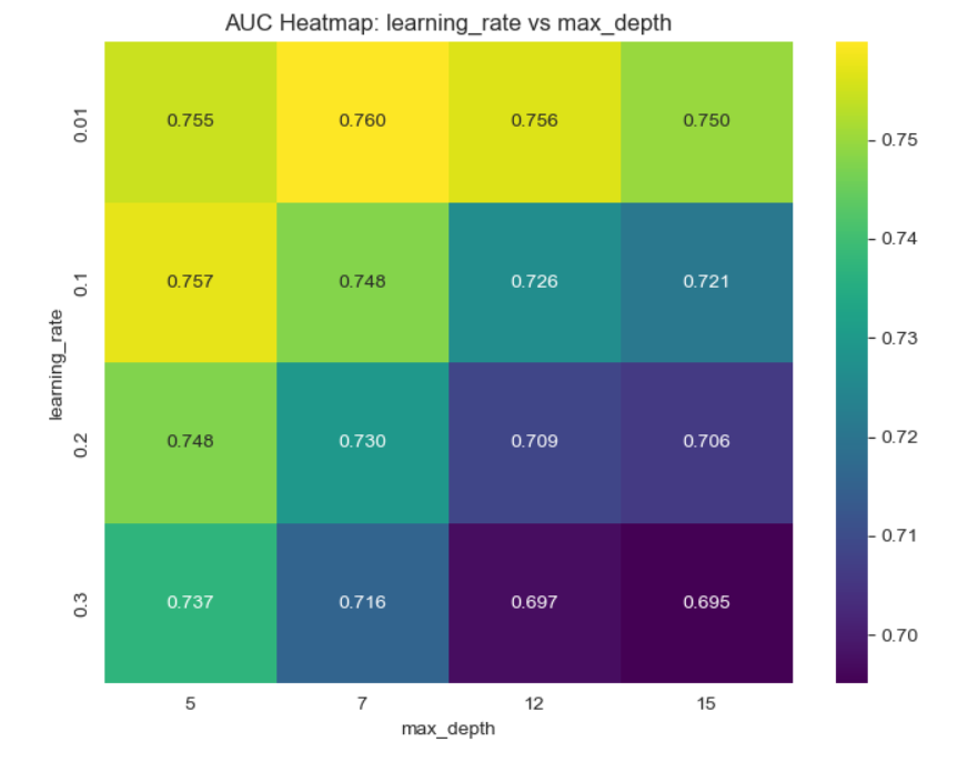
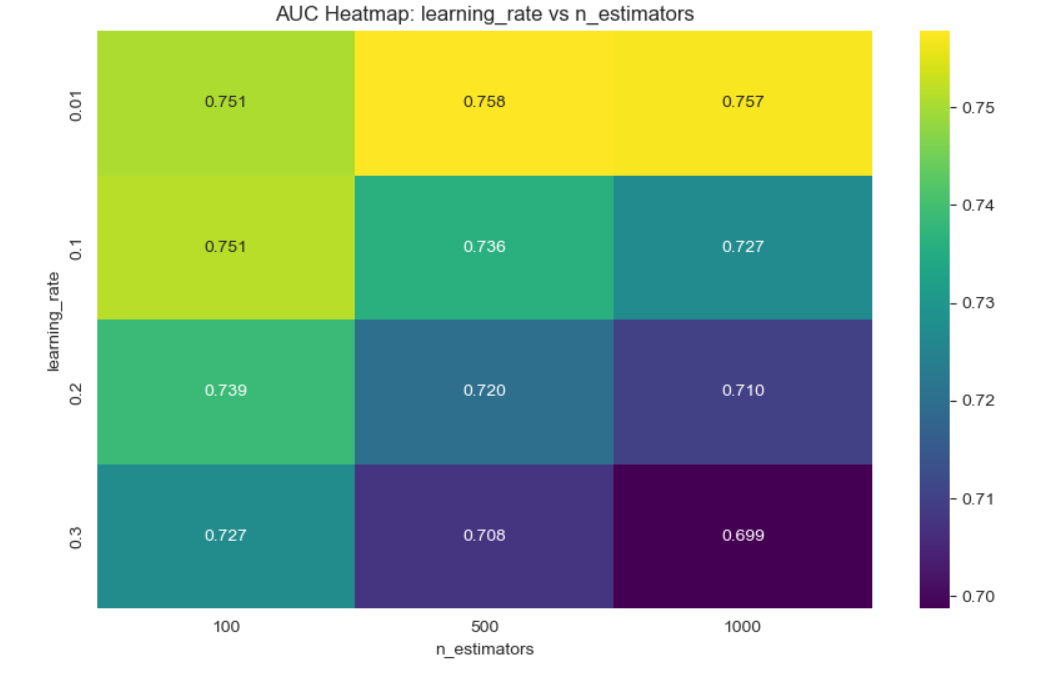
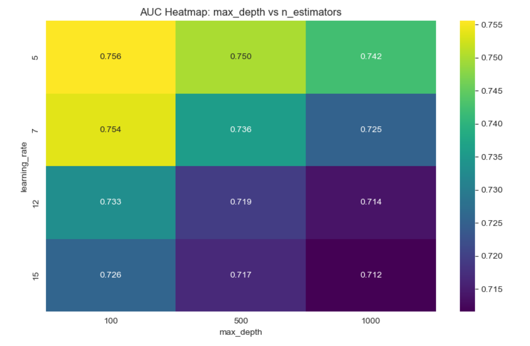
The auc score improved: auc=0.770. Accuracy is 0.931.

5.3 Feature Selection

We have explored the following techniques for feature selection:

• SelectKBest
• SelectPercentile
• RecursiveFeatureElimination
• Feature importance from tree-based models
• PCA
• SHAP

For the model, we used the simple XGBoost model without any parameters. The training and test datasets were modified to include only the features that were selected. We tried to use a variety of techniques, including filter methods, a wrapper method, an embedded method, unsupervised feature selection and to visualize the weights of the features with SHAP and a scikit method (using .plot_importance). Finally, after we had found the best selection method, we took the features it outputted and performed hyperparameter tuning on that set to see if we would obtain a better performance than the model using all the features.

Filter Methods

The two embedded methods we used were SelectKBest and SelectPercentile. Each feature is evaluated separately, ranked and the methods select the top-k or top-percentile features based on the ANOVA F-value scoring function. SelectPercentile takes the 35th percentile to return 5 features. Both methods selected the same set of features.

Wrapper Method

For the wrapper method, we tried RecursiveFeatureElimination. It starts with all features and recursively removes the least important feature in each iteration, while considering feature interactions. This method took a bit longer than the other methods to run.

Embedded Method

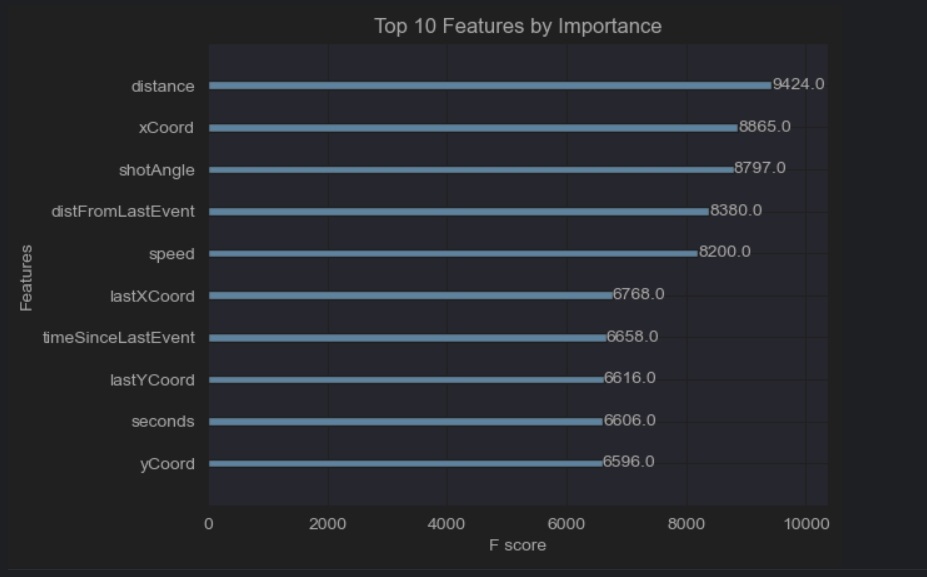
The embedded method we used was feature selection from tree-based models. XGBoost is a tree-based model which rank features based on how much they improve model performance during splits. This method aims to find the most predictive features which have higher importance scores.

Unsupervised Feature Selection

PCA was selected for the unsupervised learning method. It is useful for removing redundancy and transforms the dataset into a new set of orthogonal features by capturing the directions of maximum variance. It does not select original features but instead reduces dimensionality by retaining components that explain most of the variance.

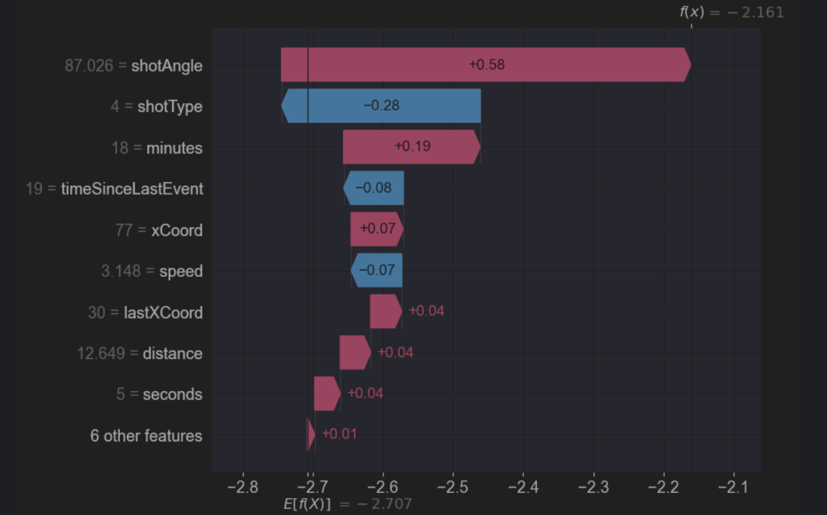
Weight Visualisation

We used the waterfall function in SHAP to visualize the weights importance of some features, which showed how much each feature contributed to the prediction compared to the baseline model. We also tried the scikit method ‘plot_importance’ and compared those results with SHAP. Although there was some overlap in the features returned, there is a discrepancy on the way the two methods seem to rank the feature’s importance.

Summary of the most important Features by Method

Here is a summary of the most important features selected by each method. For consistency, we have limited the number of features returned by each method to 5, except SHAP which has 6 features.

Technique	Features
SelectKBest	distance, shotAngle, lastEventType, rebound, speed
SelectPercentile	distance, shotAngle, lastEventType, rebound, speed
RecursiveFeatureElimination	distance, shotAngle, shotType, lastEventType, rebound
Feature importance from tree-based models	yCoord, shotType, distance, xCoord, shotAngle
PCA	distance, shotAngle, shotType, lastEventType, rebound
SHAP	‘shotAngle’, ‘minutes’, ‘xCoord’, ‘lastXCoord’, ‘distance’, ‘seconds’

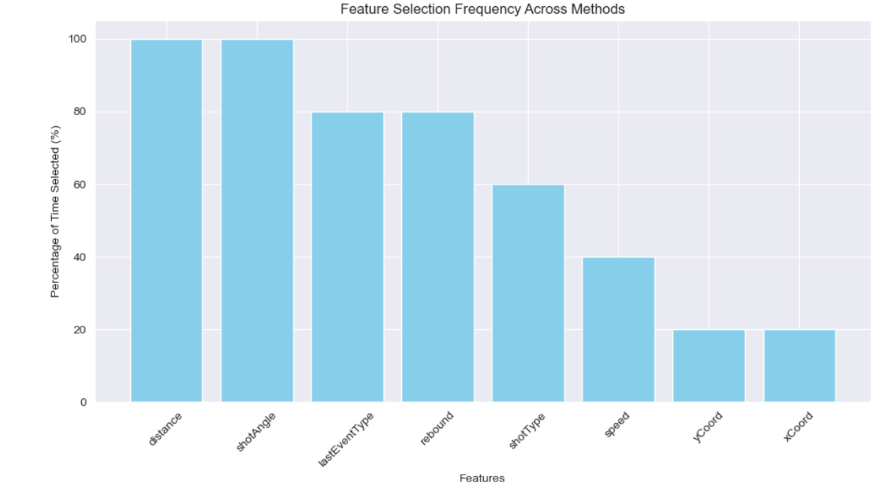
Since the features returned by each method differed, we also plotted the percentage of time a feature was selected throughout trying all these methods.

We have tried to evaluate the effect of selecting fewer features and its impact on the accuracy and the auc score. When selecting only three features with the methods specified above, we obtained the same accuracy of 0.931 while the auc score had a minimum difference of -0.01 and a maximum difference of -0.02. So, from this data, we can conclude that selecting more features will lead to a better auc score, but the added features can only improve the score so slightly.

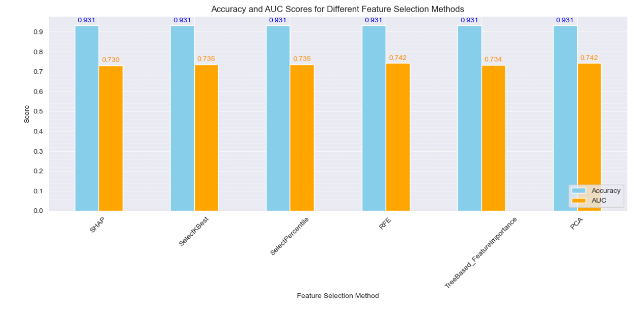
Comparison of Accuracy and AUC for each Method

We have plotted a histogram displaying the accuracy and the AUC score for each of the feature selection method. When comparing them, we can observe that

Hyperparameter Tuning with Feature Selection

After performing feature selection we choose the best model based on accuracy and AUC score. There was a tie when evaluating the best model based on AUC score: both RFE and PCA obtained 0.742. In the end, we decided to go with RFE because it is better at selecting a subset of features that are important for our specific model, and it is more interpretable. The selected features were: distance, shotAngle, shotType, lastEventType and rebound. Hyperparameter tuning was once again performed using only those features. The procedure for tuning remains the same as the previous part, with the same choices of hyperparameters. The selected feature plus the tuned hyperparameters yielded a slightly lower auc of 0.747. This might be explained by the tree structure of XGBoost which is robust to irrelevant features and performs internal feature selection.

The plots are the exact same as the previous section since it was our best overall model.

6. Give it your best shot!

For this section, we have decided to use a neural network model built with the PyTorch library.

Since our experience building neural network limited, we needed to find references and advices to configure our default neural network. We asked ChatGPT to give us a default starting point.

We came up with the following default configuration:

• Start with one fully connected hidden layer of 64x32 neurons, with ReLU activation.
• Output layer of 32x1, with Sigmoid activation to produce probabilities.
• Adam optimizer with a learning rate of 0.001.
• Perform training with 10 epochs
• Loss function Binary Cross-Entropy Loss (BCELoss in PyTorch).

6.1 Feature selection

The tidy dataset contains 10 input features (See section 4.5). We wanted to compare the performances of different selections of the 10 input features, from a small number to all of them. Note: For the categorical features (“shot type” and “last Event Type”), we have “one-hot-encoded” them before the training.

The different experiments were tracked in W&B, runs x to here: Neural Network Feature Selection experiment in W&B

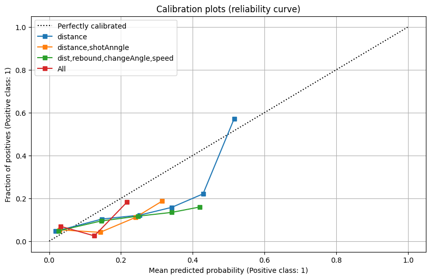In the graphs above, we observed two trends:

• Using only one feature, the distance, seems to give better results.
• Using all features seems to be equivalent to random guessing.

However, we were still interested in knowing if using more than just a single feature will give better results when we change other parameters.

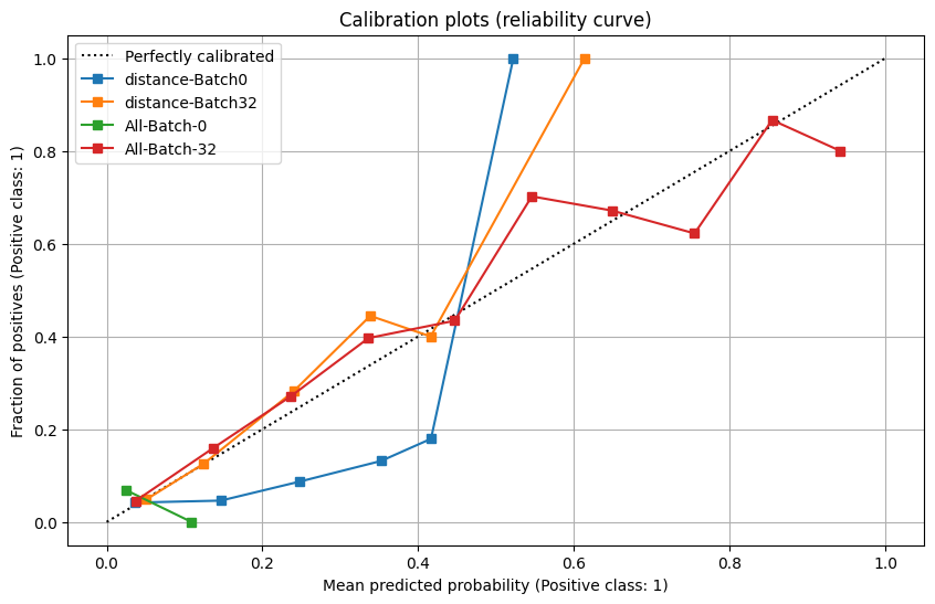
6.2. Mini-batch sizes

In the previous section, we were training our neural network on all the data set at once. For performance reasons, we know that training neural networks using mini batches should give better results in terms of computing performance and convergence.

We experimented with mini-batches sizes of 0 (no mini-batch), 32, 64, 128, 256.

Neural Network Mini-batch size experiment in W&B

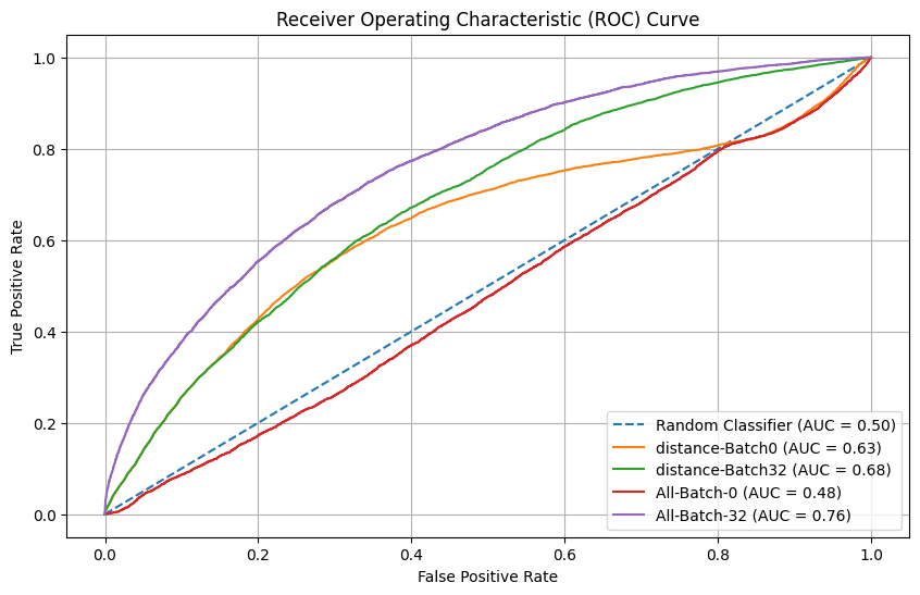
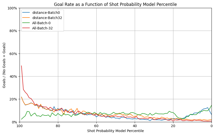
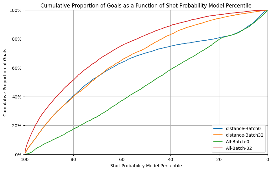
From those results, we discovered that using a mini-batch size of 32 data points seems optimal.

We decided then to compare the current experiment that used only one feature (“distance”, selected from previous section) to using all features. We made an important discovery: using all features with a mini batch of 32 gives the best results so far.

From this point, we have decided to us all 10 input features to fine-tune the following hyperparameters.

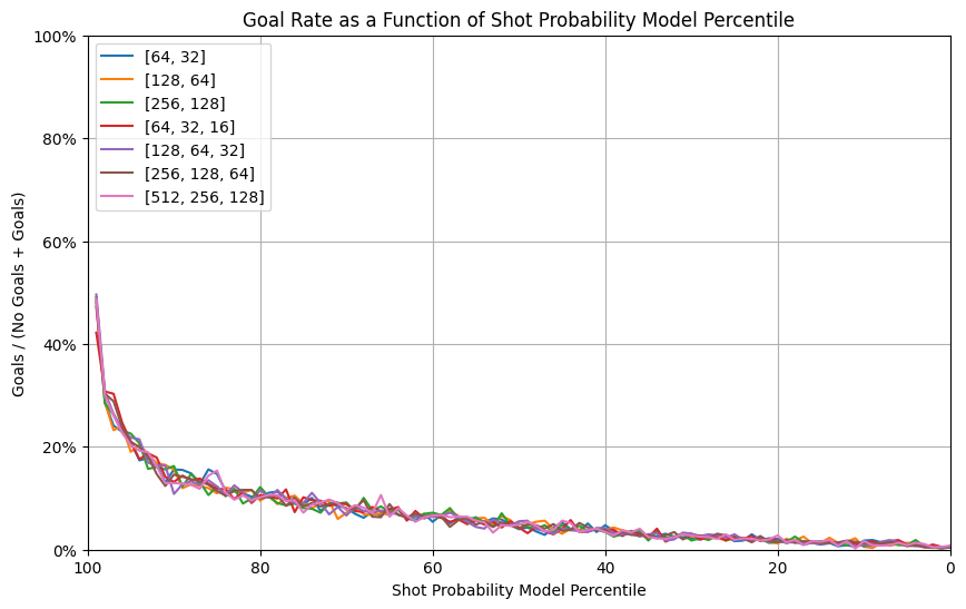
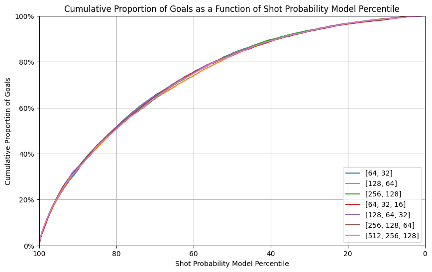
6.3. Neural Network architecture (Number of hidden layers, number of neurons)

Building from the previous section results, we wanted to test different neural network architecture on a data set using all input features and using mini batches of 32 data points. We tested the following architectures:

Number of hidden layers	Number of neurons of hidden layers
1	64x32
1	128x64
1	256x128
2	64x32, 32x16
2	128x64, 64x32
2	256x128, 128x64
2	512x128, 256x128

Neural Network Architecture experiment in W&B

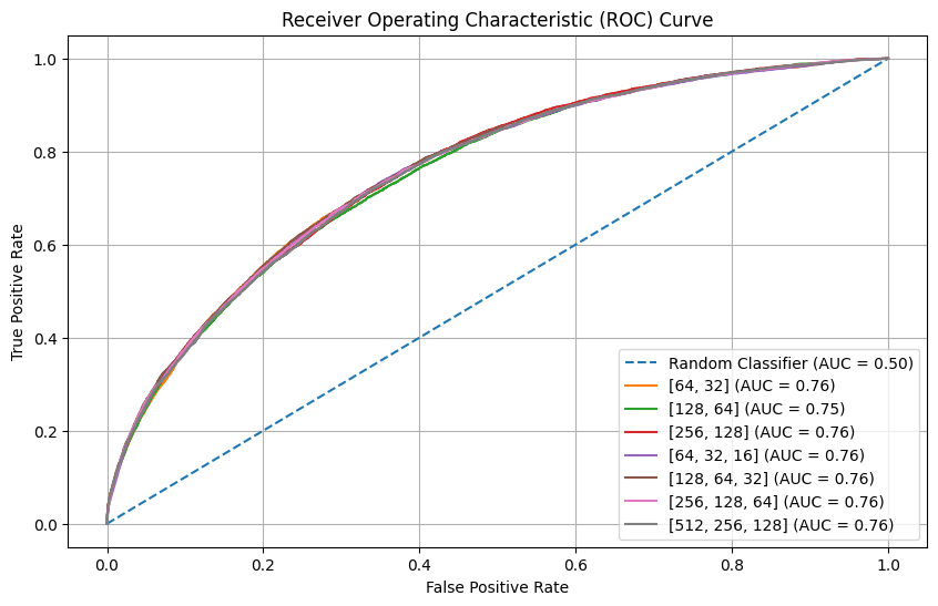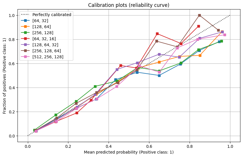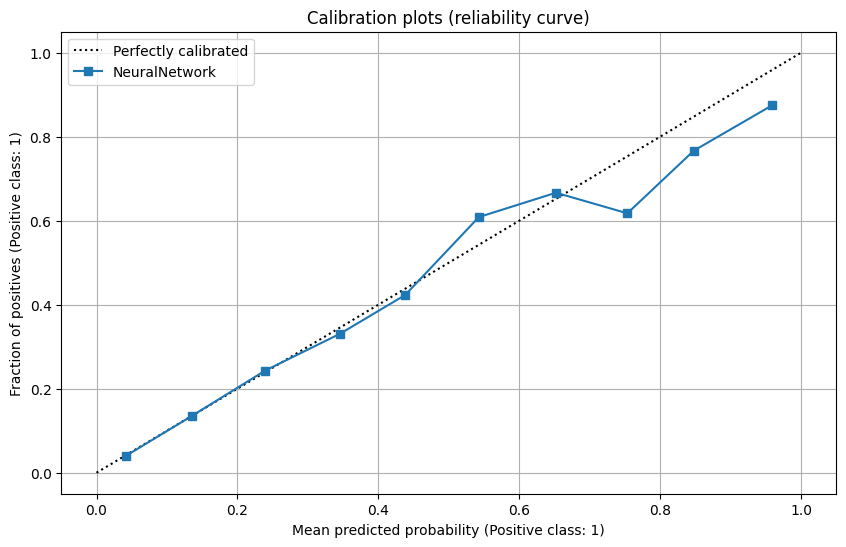
In this case, the results were surprisingly similar. There is only one graph that indicates relative differences between the architectures: the calibration plot (Reliability curve). We estimated that the curve closest to the perfectly calibrated curve is the one for the model with 2 hidden layers of 128x64 and 64x32 neurons. This seems a reasonable number of neurons with regards to the number of inputs (31 when one-hot-encode).

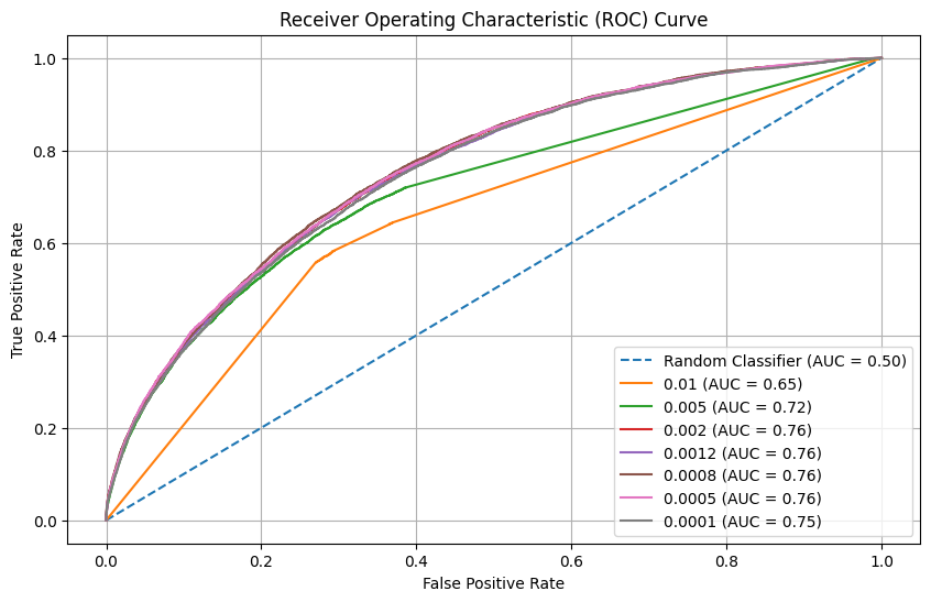
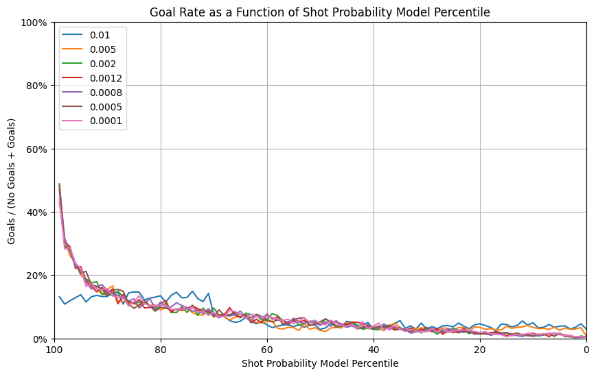
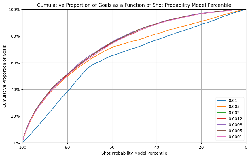
6.4 Learning rate

Learning rate can have a major impact on the performance of the model. When it is too low, we might not optimize until the minimal gradient. When too high, we might “jump” over the minimal gradient and never find it. We tested the following training rates, which are “around” our default value. 0.01, 0.005, 0.002, 0.001, 0.0008, 0.0005, 0.0001

Neural Network Learning rate experiment in W&B

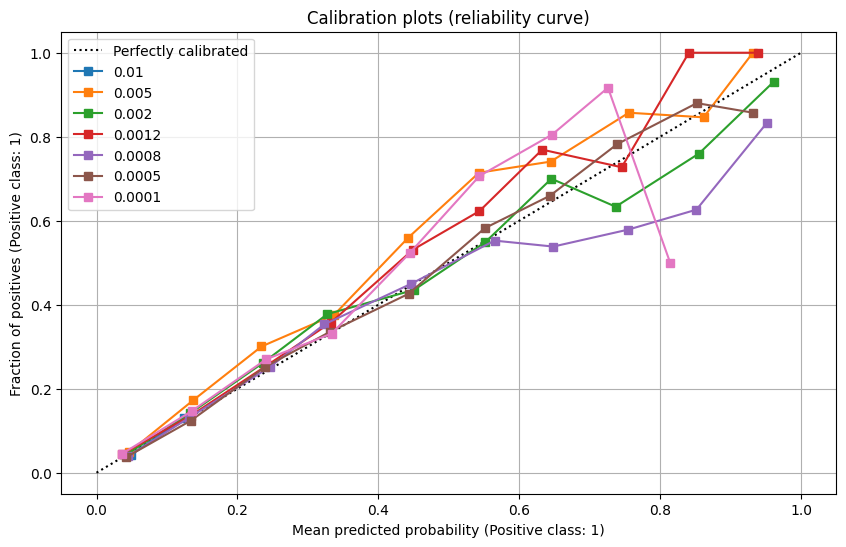We can see in the graphs above that learning rates that are too high are clearly incorrect. However, we get similar results when the learning rate is below 0.002. We have selected the best learning rate from the Calibration curve, which is 0.0005.

6.5. Number of epochs

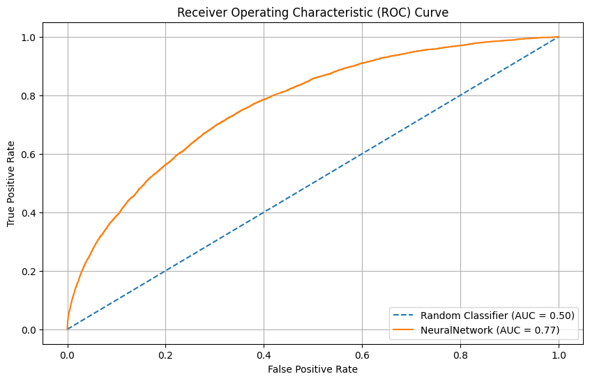
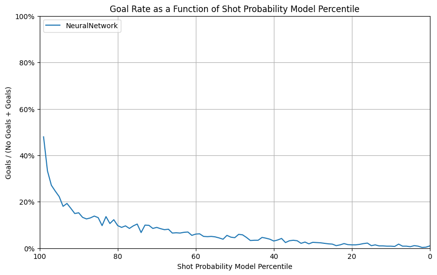
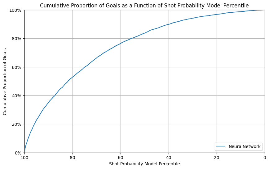
Finally, we just wanted to “push” our previous selections with a training over much more epochs. Instead of using 10 epochs, we trained our model with 100 epochs, and verified the evolution of the results (Loss, ROC AUC) during the training.

Here’s the comparison in W&B

As we can see in the results, the loss and the ROC AUC have reached a limit after 40 epochs. We will use this value for section 7.

Final Result - Our best model

• Feature Selection: use all 10 input features of Section 4.5
• Neural Network with 2 fully connected hidden layer of 128x64 and 64x32 neurons, with ReLU activation
• Output layer of 32x1, with Sigmoid activation to produce probabilities
• Training performed on mini batches of 32 data points
• Loss function Binary Cross-Entropy Loss (BCELoss in PyTorch)
• Adam optimizer with a learning rate of 0.0005
• Perform training with 100 epochs

Here’s the run result in W&B

7. Evaluate on test set

7.1 - Compare models with Test set Regular Season 2020-2021

Result for models of section 3

Logistic Regression test results on W&B

Result for models of section 5

Best XGB model on regular games

Result for model of section 6

Neural Network test results on W&B

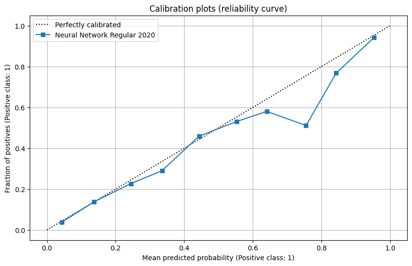Our observations:

The 3 models of logistic regression perform similarly as in the validation set, while the model with distance only has a slight improvement. Different from a distinct out-performance in models with angle in validation set, in test set experiment, all models perform similarly.

The xgb model has a similar performance as in the validation set, with a slight under-performance in calibration plot.

The NN model has a similar performance as in the validation set, with a slight under-performance in calibration plot. And comparing to xgb model, the NN model has a better performance in reliability with broader range while they have similar performance in other fields.

7.2 - Compare models with Test set Playoff Season 2020-2021

Result for models of section 3

Logistic Regression test results on W&B

Result for models of section 5

Best XGB model on playoffs

Result for model of section 6

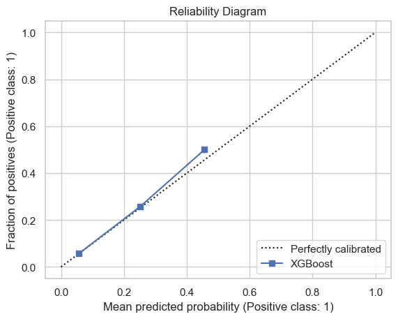
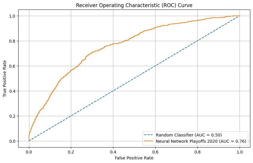
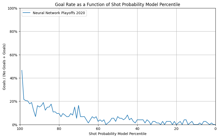
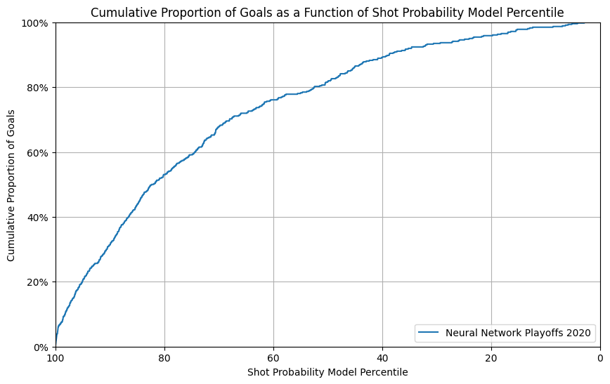
Neural Network test results on W&B

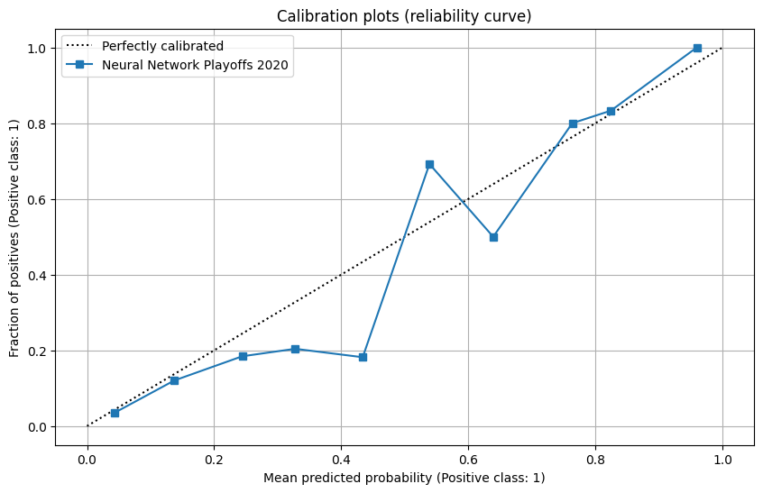Observations:

The 3 models of logistic regression perform similarly as in the regular season test set, while they have a higher variance in goal rate percentiles, suggesting a under-performance in the generalization on playoffs.

The xgb model has a similar performance as in the regular season test set, with a under-performance in goal rate percentile and calibration plot and a similar performance in reliability.

The NN model has a similar performance as in the regular season test set, with a slight under-performance in goal rate percentile and calibration plot.

Since the number of samples in playoffs are less than regular season, the generalization might have a higher variance.